Universal Downscaling Task: Model Evaluation and Comparison

The universal downscaling task considers the GLM model, where 81 separate GLMs are constructed to predict each of the target global solar radiation grid points, and the CNN-LSTM_U architecture, where grid points for all GCM predictors (except prsn and plev variables having missing data) are provided as inputs and all 81 radiation grid points are generated by the network output (as shown in Figure 24). Both sites Springs and Mossman South Alchera Drive were excluded from the data set due to missing data for some of the target grid points, leaving a remaining 16 sites available for evaluation. The configuration of the CNN-LSTM_U architecture resulted after a preliminary grid search, which narrowed the choices for the CNN filter configuration and the final candidate was selected after fine tuning loss functions and learning rate as described in Table 12. Metrics are calculated for each of the 81 grid points by converting from a matrix into a single vector and combining all vectors for the date range in the held-out test period.

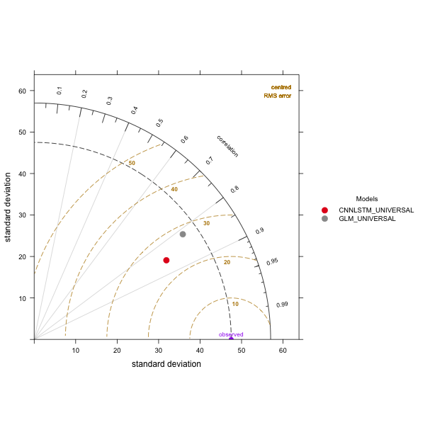
Figure 49 Taylor diagram comparing GLM_UNIVERSAL and CNN-LSTM UNIVERSAL models.

The CNN-LSTM_U model exhibits slightly higher correlation and less RMSE than the GLM model as illustrated by the Taylor diagram in Figure 49, however the standard deviation is less than that of the observed data. The lower mean and standard deviation are penalised by the Kling-Gupta Efficiency for the CNN-LSTM_U where the GLM model exhibits a better score for the majority of sites (Table 22). For example, the overall mean of the observations across all grid points and sites is \(228Wm^{- 2}\) whereas the overall standard deviation is \(47.27Wm^{- 2}\), in comparison the simulation for the CNN-LSTM_U has overall mean and standard deviation of \(223.74Wm^{- 2}\) and \(37.14Wm^{- 2}\) respectively, and similarly for the GLM, \(229.07Wm^{- 2}\) and \(43.9Wm^{- 2}\). This result is in contrast to the other metrics where the CNN-LSTM_U exhibits better performance for all sites except Carpentaria Downs Station and Majors Creek. The CNN-LSTM_U model exhibits higher \(R^{2}\) for the majority of sites with the highest metric of 0.83 for Harewood and Mount Larcom Post Office and the lowest of 0.57 at Carpentaria Downs Station (Table 23). While the GLM model exhibits highest \(R^{2}\) for the Harewood site of 0.74 and the minimum \(R^{2}\) at Carpentaria Downs Station of 0.52. Willmott’s index of Agreement is higher for the GLM for four of the observation sites, with the highest value being for Woolooga at a 0.92 and lowest of 0.83 for Carpentaria Downs Station (Table 23). The CNN-LSTM_U model exhibits higher agreement for the majority of the sites, with the maximum being 0.94 at Mount Larcom Post Office and the lowest at the Carpentaria Downs Station of 0.77. The GLM model demonstrates a higher Nash-Sutcliffe Efficiency for three sites with the maximum being 0.73 for sites Harewood and minimum of 0.32 at Carpentaria Downs Station (Table 22). Maximum value of efficiency is achieved by the CNN-LSTM_U model is for the Mount Larcom Post Office at 0.81 with the minimum being 0.13 at Carpentaria Downs Station. Results for the RMSE indicate that the GLM model has lower RMSE for Carpentaria Downs Station and Majors Creek with the minimum RMSE given for Woolooga at 24.43 \(Wm^{- 2}\) and the maximum RMSE at Wooleebee Nevasa of 39.54 \(Wm^{- 2}\) (Table 24). The CNN-LSTM_U model has lower RMSE for the remaining sites with Mount Larcom Post Office having the smallest RMSE at 19.43 \(Wm^{- 2}\) and the largest at Carpentaria Downs Station with 36.27 \(Wm^{- 2}\). Maximum value for MAE produced by the GLM model also correspond to the Wooleebee Nevasa site at 31.20 \(Wm^{- 2}\)and the minimum produced at Mount Larcom Post Office of 19.9 \(Wm^{- 2}\) (Table 24). The \(CNN - LSTM_{U}\) exhibits a minimum MAE at Mount Larcom Post Office at 15.25 \(Wm^{- 2}\) and the maximum of 31 \(Wm^{- 2}\ \)at Carpentaria Downs Station. The RRMSE for the GLM model resides within the 10% - 20% interval with the best value at Glenlands of 10.83% and largest at Woleebee Nevasa of 17.23% (Table 25). A number of sites for the CNN-LSTM_U model exhibit a RRMSE below 10% with the best score at Mount Larcom Post office of 8.43%. The worst RRMSE score for the CNN-LSTM_Umodel is for the Carpentaria Downs Station at 15.43%.

Table 22 Kling-Gupta Efficiency and Nash-Sutcliffe Efficiency per site for the universal downscaling task. Values in bold indicate better scores.

	Kling-Gupta Efficiency		Nash-Sutcliffe Efficiency
Site	CNN-LSTM_U	GLM	CNN-LSTM_U	GLM
Barmount	0.77	0.78	0.69	0.63
Carpentaria Downs Station	0.71	0.70	0.13	0.32
Comet Post Office	0.76	0.81	0.67	0.64
Glenlands	0.81	0.82	0.79	0.68
Harewood	0.71	0.79	0.79	0.73
Majors Creek	0.77	0.80	0.55	0.59
Miles Post Office	0.71	0.80	0.79	0.73
Mount Larcom Post Office	0.81	0.79	0.81	0.66
New Caledonia	0.78	0.81	0.70	0.65
Riverview Hopeland	0.72	0.77	0.79	0.72
Talagai	0.77	0.78	0.66	0.60
Woleebee Nevasa	0.72	0.78	0.78	0.39
Woolooga	0.76	0.84	0.72	0.72

Table 23 Comparison of \(R^{2}\) and Willmott’s index of Agreement for universal models. Values in bold indicate better scores.

	\(\mathbf{R}^{\mathbf{2}}\)		Willmott’s Index of Agreement
Site	CNN-LSTM_U	GLM	CNN-LSTM_U	GLM
Barmount	0.74	0.64	0.90	0.89
Carpentaria Downs Station	0.57	0.52	0.77	0.83
Comet Post Office	0.74	0.67	0.90	0.90
Glenlands	0.82	0.70	0.93	0.91
Harewood	0.83	0.74	0.93	0.92
Majors Creek	0.68	0.64	0.87	0.89
Miles Post Office	0.82	0.73	0.93	0.92
Mount Larcom Post Office	0.83	0.68	0.94	0.90
New Caledonia	0.75	0.67	0.91	0.90
Riverview Hopeland	0.82	0.73	0.93	0.91
Talagai	0.73	0.64	0.90	0.88
Woleebee Nevasa	0.81	0.65	0.92	0.85
Woolooga	0.80	0.73	0.91	0.92

Table 24 Comparison of Root Mean Square Error (RMSE) and Mean Absolute Error (MAE) for universal models. Values in bold indicate better scores.

	RMSE \(\mathbf{W}\mathbf{m}^{\mathbf{- 2}}\)		MAE \(\mathbf{W}\mathbf{m}^{\mathbf{- 2}}\)
Site	CNN-LSTM_U	GLM	CNN-LSTM_U	GLM
Barmount	24.75	27.27	19.66	20.90
Carpentaria Downs Station	36.27	31.99	31.00	24.40
Comet Post Office	25.63	26.87	20.29	20.51
Glenlands	20.59	25.13	16.20	19.56
Harewood	23.45	26.44	18.59	21.25
Majors Creek	28.06	26.82	23.36	21.22
Miles Post Office	23.65	26.49	18.76	20.89
Mount Larcom Post Office	19.43	25.74	15.25	19.90
New Caledonia	24.40	26.30	19.28	19.94
Riverview Hopeland	23.15	26.69	18.28	21.20
Talagai	25.81	28.11	20.63	22.16
Woleebee Nevasa	23.85	39.54	18.86	31.20
Woolooga	24.39	24.43	18.82	19.28

Table 25 Comparison of Relative Root Mean Square Error (RRMSE) for universal models. Values in bold indicate better scores.

	RRMSE %
Site Name	CNN-LSTM_U	GLM
Barmount	10.74	11.81
Carpentaria Downs Station	15.43	13.58
Comet Post Office	11.09	11.60
Glenlands	8.89	10.83
Harewood	10.3	11.59
Majors Creek	12.11	11.56
Miles Post Office	10.38	11.60
Mount Larcom Post Office	8.43	11.14
New Caledonia	10.55	11.35
Riverview Hopeland	10.21	11.75
Talagai	11.15	12.12
Woleebee Nevasa	10.42	17.23
Woolooga	11.17	11.16

The best performing metrics for the CNN-LSTM_Umodel include sites Glenlands and Mount Larcom Post Office, while the worst performing metrics are identified as Carpentaria Downs Station.

In comparing the bias for Mount Larcom Post Office, the histogram in Figure 50 indicates that the CNN-LSTM_Uto be slightly more normally distributed in comparison to the GLM model with a slightly wider spread of bias between -60 and 60 \(Wm^{- 2}\).

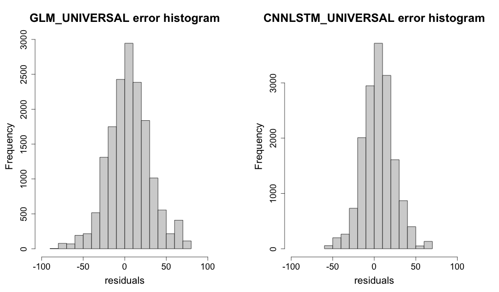
Figure 50 Histogram of the residual error \(Wm^{- 2}\) for all predictions at Mount Larcom Post Office.

Both models appear to exhibit general extremes of higher absolute bias during the summer months and in general minimums appear to occur during the winter months. Mean values for the error per month of year indicate higher values for January – March with the CNN-LSTM_U model exhibiting a lower overall range of mean errors between -9.2\(Wm^{- 2}\) to 17.7\(Wm^{- 2}\) as opposed to the GLM model with mean errors in the range of -12.\(5Wm^{- 2}\) to 26.9\(Wm^{- 2}\) (Figure 51).

table>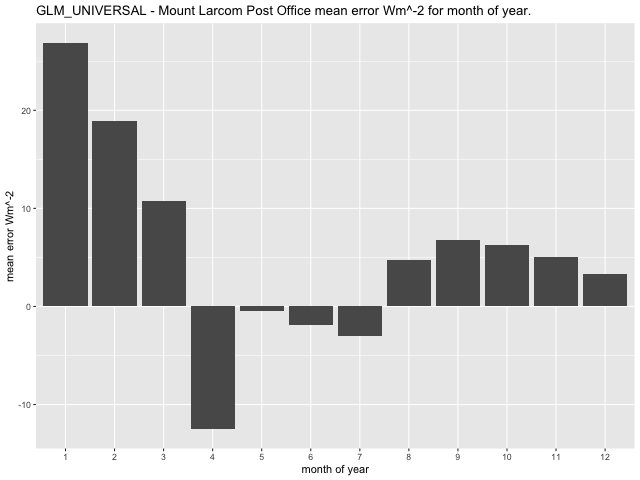

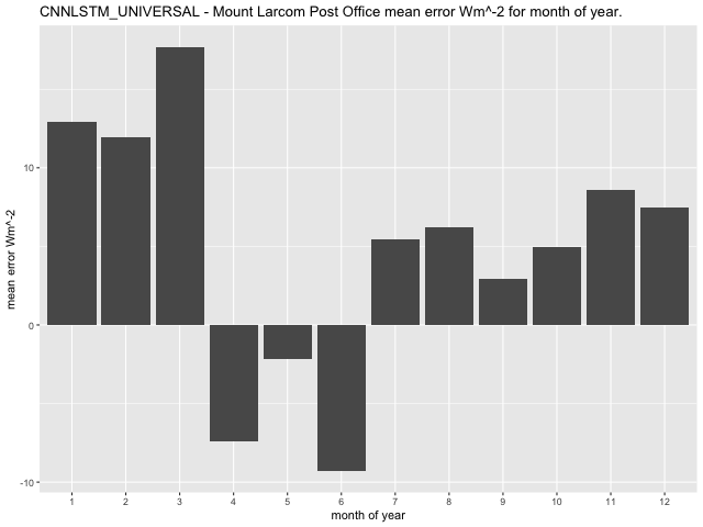
Figure 51 Comparison of mean error \(Wm^{- 2}\) for month of year at Mount Larcom Post Office.

Comparing the distribution for bias at the site Carpentaria Downs Station, Figure 52 indicates difference in means between the residuals for the GLM and CNN-LSTM_Uwith the latter having mean residuals for this site closer to 40\(Wm^{- 2}\), as opposed to errors for the GLM model appear to be closer to a mean of \(0Wm^{- 2}\) between \(- 100Wm^{- 2}\) and \(- 60Wm^{- 2}\).

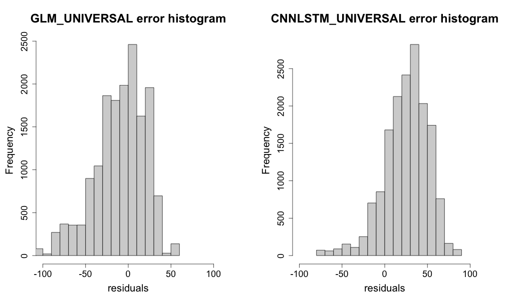
Figure 52 Histogram of residuals in \(Wm^{- 2}\) at Carpentaria Downs Station for both models.

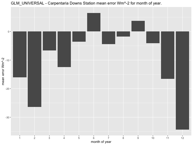
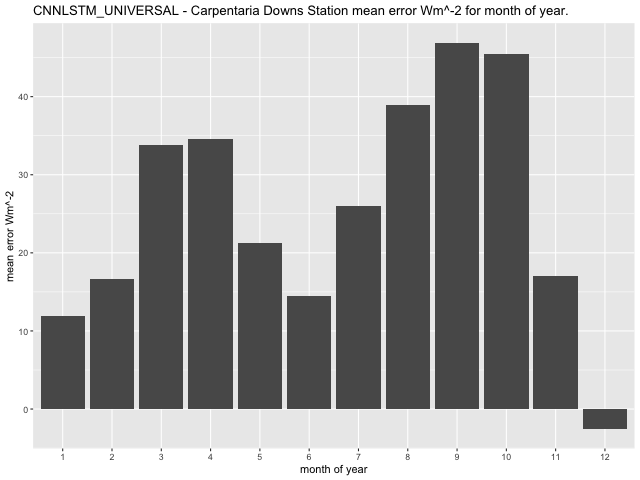
Higher extremes of bias at the Carpentaria Downs Station also appear to occur during the summer months for the GLM and during early Autumn and Spring for the CNN-LSTM_Umodel. Reviewing Figure 53 the range of the mean error for the GLM model per month is lower (-34.34\(\text{\ W}m^{- 2}\) to 6.55\(\text{\ W}m^{- 2}\)) than that of the CNN-LSTM_Umodel (-2.58\(\text{\ W}m^{- 2}\) to 46.93 \(Wm^{- 2}\)) at this site with the GLM reflecting larger mean error in Summer (February, December) while the CNN-LSTM_Ureflects a larger mean error in early Autumn (March, April) and Spring (September, October).

Figure 53 Comparison of mean error \(Wm^{- 2}\) for month of year at Comet Post Office.

Future Scenario RCP4.5 2006 to 2020

In most locations under the RCP4.5 climate warming scenario, the CNN-LSTM universal model demonstrates better performance on the evaluation metrics for the period 2006 to 2020. The exceptions occur in the KGE metric for the sites Harewood, Miles Post Office, Riverview Hopeland, Talagai and Woolooga where the GLM exhibits a higher KGE.

Table 26 Evaluation metrics under the RCP4.5 profile for both universal models 2006 to 2020. Values in bold indicate better scores.

Site Name	Model Name	KGE	E	\[\mathbf{R}^{\mathbf{2}}\]	d	RMSE \(\mathbf{W}\mathbf{m}^{\mathbf{- 2}}\)	MAE \(\mathbf{W}\mathbf{m}^{\mathbf{- 2}}\)	RRMSE %
Barmount	CNN-LSTM_U	0.76	0.70	0.71	0.90	22.77	17.32	10.80
	GLM	0.74	-0.19	0.68	0.76	48.65	41.76	22.05

Carpentaria Downs Station	CNN-LSTM_U	0.81	0.64	0.68	0.90	21.50	17.88	9.88
	GLM	0.71	-0.63	0.63	0.71	49.14	42.10	21.57

Comet Post Office	CNN-LSTM_U	0.76	0.73	0.74	0.91	21.72	16.99	10.11
	GLM	0.75	-0.11	0.68	0.76	47.74	40.90	21.21

Glenlands	CNN-LSTM_U	0.77	0.71	0.74	0.91	22.19	16.93	10.59
	GLM	0.74	-0.16	0.68	0.76	47.96	40.99	21.88

Harewood	CNN-LSTM_U	0.70	0.77	0.82	0.92	22.71	18.24	10.73
	GLM	0.78	0.15	0.78	0.81	47.15	41.24	21.30

Majors Creek	CNN-LSTM_U	0.77	0.67	0.67	0.90	22.45	17.63	10.62
	GLM	0.72	-0.42	0.65	0.73	49.75	42.96	22.48

Miles Post Office	CNN-LSTM_U	0.70	0.77	0.81	0.92	22.60	18.07	10.64
	GLM	0.77	0.18	0.76	0.81	46.05	39.08	20.72

Mount Larcom Post Office	CNN-LSTM_U	0.78	0.70	0.76	0.91	22.32	17.01	10.76
	GLM	0.73	-0.33	0.69	0.73	50.71	44.12	23.36

New Caledonia	CNN-LSTM_U	0.76	0.73	0.73	0.91	21.89	17.00	10.26
	GLM	0.74	-0.10	0.67	0.77	47.27	39.89	21.17

Riverview Hopeland	CNN-LSTM_U	0.71	0.76	0.82	0.92	22.78	18.29	10.81
	GLM	0.77	0.17	0.78	0.81	46.02	39.97	20.88

Talagai	CNN-LSTM_U	0.75	0.72	0.72	0.91	22.25	17.26	10.43
	GLM	0.76	0.04	0.67	0.79	44.07	37.22	19.74

Woleebee Nevasa	CNN-LSTM_U	0.71	0.76	0.80	0.92	22.55	17.91	10.60
	GLM	0.66	-0.67	0.67	0.71	64.65	56.39	29.02

Woolooga	CNN-LSTM_U	0.73	0.62	0.78	0.88	27.02	21.52	13.39
	GLM	0.74	-0.15	0.73	0.76	50.51	44.38	23.94

Future Scenario RCP8.5 2006 to 2020

Under the RCP8.5 climate warming scenario, the KGE demonstrate better performance of the GLM model at a majority of sites similar to the test set. However, the CNN-LSTM_U exhibits good performance for all other metrics as shown in Table 27.

Table 27 Evaluation metrics under the RCP8.5 profile for both universal models 2006 to 2020. Values in bold indicate better scores.

Site Name	Model Name	KGE	E	\[\mathbf{R}^{\mathbf{2}}\]	d	RMSE \(\mathbf{W}\mathbf{m}^{\mathbf{- 2}}\)	MAE \(\mathbf{W}\mathbf{m}^{\mathbf{- 2}}\)	RRMSE %
Barmount	CNN-LSTM_U	0.76	0.70	0.71	0.91	22.73	17.34	10.79
	GLM	0.77	0.59	0.64	0.88	28.54	22.28	12.94

Carpentaria Downs Station	CNN-LSTM_U	0.82	0.66	0.69	0.90	21.00	17.35	9.66
	GLM	0.74	0.29	0.58	0.82	32.36	26.21	14.20

Comet Post Office	CNN-LSTM_U	0.76	0.74	0.74	0.92	21.56	16.78	10.03
	GLM	0.81	0.64	0.69	0.90	27.34	20.90	12.15

Glenlands	CNN-LSTM_U	0.77	0.71	0.74	0.91	22.27	17.03	10.63
	GLM	0.79	0.58	0.64	0.88	28.87	21.71	13.17

Harewood	CNN-LSTM_U	0.70	0.77	0.82	0.92	22.74	18.25	10.75
	GLM	0.81	0.70	0.75	0.91	27.81	21.60	12.56

Majors Creek	CNN-LSTM_U	0.78	0.67	0.68	0.90	22.26	17.39	10.53
	GLM	0.75	0.47	0.58	0.85	30.30	23.82	13.70

Miles Post Office	CNN-LSTM_U	0.70	0.77	0.81	0.92	22.59	18.07	10.64
	GLM	0.83	0.76	0.76	0.93	24.96	19.19	11.23

Mount Larcom Post Office	CNN-LSTM_U	0.78	0.70	0.76	0.91	22.42	17.10	10.80
	GLM	0.74	0.58	0.62	0.87	28.56	21.88	13.15

New Caledonia	CNN-LSTM_U	0.76	0.73	0.73	0.91	21.75	16.85	10.20
	GLM	0.80	0.62	0.67	0.89	27.68	21.43	12.40

Riverview Hopeland	CNN-LSTM_U	0.71	0.76	0.82	0.92	22.79	18.32	10.82
	GLM	0.79	0.72	0.75	0.91	26.83	20.81	12.17

Talagai	CNN-LSTM_U	0.76	0.72	0.72	0.91	22.09	17.12	10.35
	GLM	0.81	0.67	0.68	0.91	25.92	19.26	11.61

Woleebee Nevasa	CNN-LSTM_U	0.71	0.77	0.80	0.92	22.49	17.86	10.57
	GLM	0.77	0.31	0.65	0.83	41.49	34.00	18.62

Woolooga	CNN-LSTM_U	0.73	0.61	0.78	0.88	27.32	21.82	13.54
	GLM	0.80	0.59	0.67	0.89	30.17	23.47	14.30

Chapter 4: Model Evaluation and Comparison

Universal Downscaling Task: Model Evaluation and Comparison

Future Scenario RCP4.5 2006 to 2020

Future Scenario RCP8.5 2006 to 2020