Chapter 3: Data Preparation
GCM Ensemble Model Creation by Model Aggregation
The following diagram illustrates the process by which the GCM model outputs were averaged between 3 selected GCM models (i.e., ACCESS1-0, HadGEM2-CC and MRI-CGCM3) in order to produce the predictor variable dataset used in modelling the global solar radiation on ground level. The first step applied a filter to select GCM outputs from within the QLD state region using the bounding box formed by longitudes 136 to 155 and latitudes -8.5 to -30. As the MRI-CGCM3 model produced outputs at a slightly different grid resolution to the other two models, the second step applied an inverse distance weighting interpolation (the “idw” routine is provided by the R package “gstat” [1] [2] to the filtered MRI-CGCM3 outputs, using the reference grid derived from the ACCESS1-0 filtered data set. This resulted in the re-gridded MRI-CGCM3 data set that was then able to be combined with the other two filtered outputs to calculate an ensemble average for the QLD region.
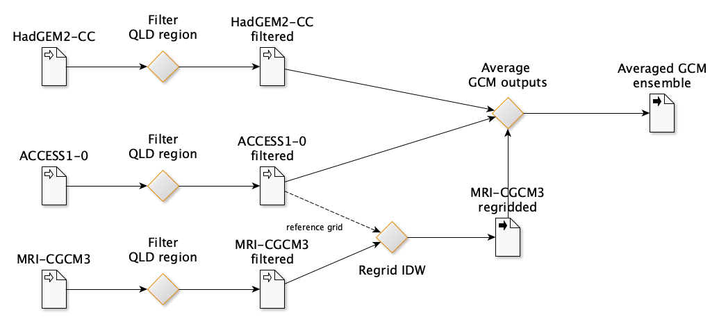
Figure 4 Ensemble data produced from averaging GCM outputs.
Mappings between GCM grid points and SILO observation sites
The resulting ensemble data set was then used as the input for site selection, were data points for each of the mapped observation sites were extracted for subsequent modelling using the closest data point given by the haversine distance between the coordinates of the GCM grid point and the mapped observation site.
The following table (Table 5) lists the set of SILO observation sites and the corresponding distances from the nearest GCM grid point.
The grid dimension of the GCM model is 1.25 x 1.875 degrees approximately 250km x 250km. The distance to the site for the closest point is required to be approximately less than 125km. Note that as there are a number of sites which share the same GCM grid point, those sites which are furthest from the grid point are selected for removal from the data set. These are shown in Table 5 as those rows associated with an asterisk.
| SILO Site | Site lon \(\mathbf{{^\circ}}\) | Site lat \(\mathbf{{^\circ}}\) | GCM lon \(\mathbf{{^\circ}}\) | GCM lat \(\mathbf{{^\circ}}\) | Distance to site km |
|---|---|---|---|---|---|
| Barmount | 149.10\({^\circ}E\) | 22.53\({^\circ}S\) | 150.00\({^\circ}E\) | 22.50\({^\circ}S\) | 86.80 |
| Carpentaria Downs Station | 144.32\({^\circ}E\) | 18.72\({^\circ}S\) | 144.38\({^\circ}E\) | 18.75\({^\circ}S\) | 6.17 |
| Comet Post Office | 148.54\({^\circ}E\) | 23.60\({^\circ}S\) | 148.13\({^\circ}E\) | 23.75\({^\circ}S\) | 42.89 |
| Glenlands | 150.51\({^\circ}E\) | 23.53\({^\circ}S\) | 150.00\({^\circ}E\) | 23.75\({^\circ}S\) | 55.01 |
| Harewood | 150.47\({^\circ}E\) | 26.92\({^\circ}S\) | 150.00\({^\circ}E\) | 27.50\({^\circ}S\) | 79.10 |
| Majors Creek | 146.93\({^\circ}E\) | 19.60\({^\circ}S\) | 146.25\({^\circ}E\) | 20.00\({^\circ}S\) | 77.83 |
| Miles Post Office | 150.18\({^\circ}E\) | 26.66\({^\circ}S\) | 150.00\({^\circ}E\) | 26.25\({^\circ}S\) | 48.74 |
| Mossman South Alchera Drive | 145.37\({^\circ}E\) | 16.47\({^\circ}S\) | 146.25\({^\circ}E\) | 16.25\({^\circ}S\) | 84.22 |
| Mount Larcom Post office | 150.98\({^\circ}E\) | 23.81\({^\circ}S\) | 151.88\({^\circ}E\) | 23.75\({^\circ}S\) | 87.82 |
| New Caledonia | 148.93\({^\circ}E\) | 23.43\({^\circ}S\) | 148.13\({^\circ}E\) | 23.75\({^\circ}S\) | 84.02 |
| Riverview Hopeland | 150.69\({^\circ}E\) | 26.81\({^\circ}S\) | 150.00\({^\circ}E\) | 26.25\({^\circ}S\) | 91.41 |
| Springs | 151.51\({^\circ}E\) | 24.17\({^\circ}S\) | 151.88\({^\circ}E\) | 23.75\({^\circ}S\) | 58.32 |
| Talagai | 148.53\({^\circ}E\) | 23.13\({^\circ}S\) | 148.13\({^\circ}E\) | 23.75\({^\circ}S\) | 78.42 |
| Woleebee Nevasa | 149.83\({^\circ}E\) | 26.29\({^\circ}S\) | 150.00\({^\circ}E\) | 26.25\({^\circ}S\) | 16.98 |
| Woolooga | 152.39\({^\circ}E\) | 26.05\({^\circ}S\) | 151.88\({^\circ}E\) | 26.25\({^\circ}S\) | 55.34 |
Table 5 Mapping between observation site and ensembled GCM grid point.
SILO observations for radiation are then converted from \(\text{MJ}m^{- 2}\text{da}y^{- 1}\) into \(Wm^{- 2}\) so as to equate the observed global solar radiation with that of the GCM model outputs (\(1Wm^{- 2} \times 0.000001J \times \left( 60 \times 60 \times 24 \right)s = 0.0864MJm^{- 2}\text{da}y^{- 1}\)).
In the case of 2-dimensional data, nine closest grid points for each date (forming a 3x3 grid) are selected for each site from the ensemble outputs for each GCM variable. Figure 5 illustrates the source data grid at the observation station Carpentaria Downs Station with the GCM output “rsds.” A separate grid is extracted for each of the GCM outputs and are combined for the 2-dimensional modelling task. For the SILO data the closest 81 grid points around the observation site are selected for each date, forming a 9x9 grid for the target downscaling. Figure 6 illustrates the target grid at the observation station Carpentaria Downs Station. A subset of the sites are then processed in the 2-dimensional setting due to missing data for some sites.
p>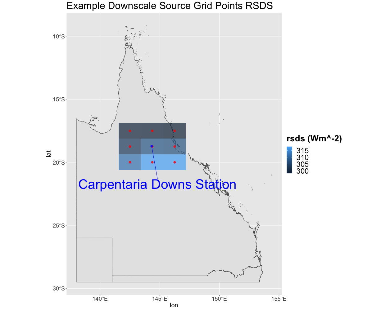
Figure 5 An example 3x3 grid for the GCM variable rsds shown for the observation station Carpentaria Downs Station.
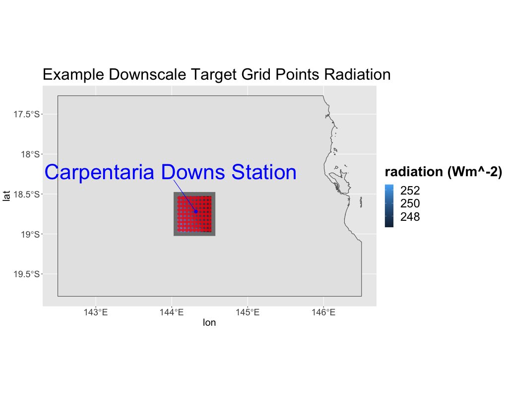
Figure 6 Example of the 9x9 target observation grid of observed global solar radiation for the Carpentaria Downs observation station.
Cross Correlation of Predicator Variables against SILO Radiation
Correlation between daily radiation and GCM predictors are lower than the month averaged radiation and GCM predictors. Both timescales exhibit similar seasonal correlation with radiation. Periods of strong correlation appear to be up to 100 days for day resolution data and up to a period of 6 months for month resolution data. The following figures (Figure 7 to Figure 18) illustrate the cross correlation between the predictors and the target radiation variable at the Barmount observation site. The modelling leveraged monthly averages for each of the target sites.
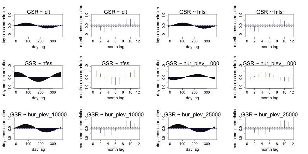
Figure 7 Comparison of daily cross correlation with monthly average cross correlation for each GCM variable against global solar radiation (GSR) at each time scale for the Barmount site.
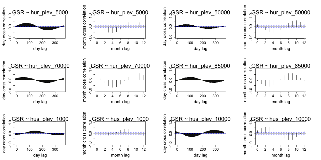
Figure 8 Comparison of daily cross correlation with monthly average cross correlation for each GCM variable against global solar radiation (GSR) at each time scale for the Barmount site.
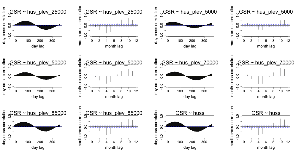
Figure 9 Comparison of daily cross correlation with monthly average cross correlation for each GCM variable against global solar radiation (GSR) at each time scale for the Barmount site.
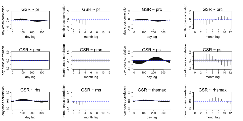
Figure 10 Comparison of daily cross correlation with monthly average cross correlation for each GCM variable against global solar radiation (GSR) at each time scale for the Barmount site.
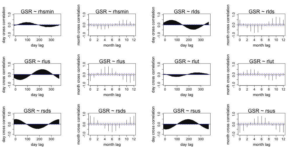
Figure 11 Comparison of daily cross correlation with monthly average cross correlation for each GCM variable against global solar radiation (GSR) at each time scale for the Barmount site.
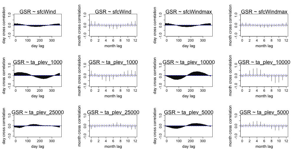
Figure 12 Comparison of daily cross correlation with monthly average cross correlation for each GCM variable against global solar radiation (GSR) at each time scale for the Barmount site.
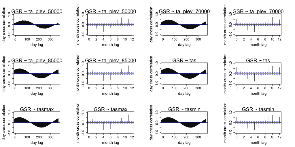
Figure 13 Comparison of daily cross correlation with monthly average cross correlation for each GCM variable against global solar radiation (GSR) at each time scale for the Barmount site.
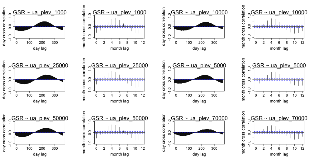
Figure 14 Comparison of daily cross correlation with monthly average cross correlation for each GCM variable against global solar radiation (GSR) at each time scale for the Barmount site.
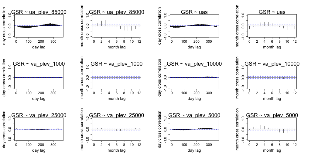
Figure 15 Comparison of daily cross correlation with monthly average cross correlation for each GCM variable against global solar radiation (GSR) at each time scale for the Barmount site.
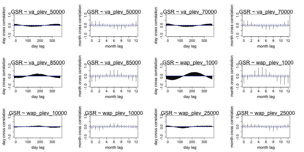
Figure 16 Comparison of daily cross correlation with monthly average cross correlation for each GCM variable against global solar radiation (GSR) at each time scale for the Barmount site.
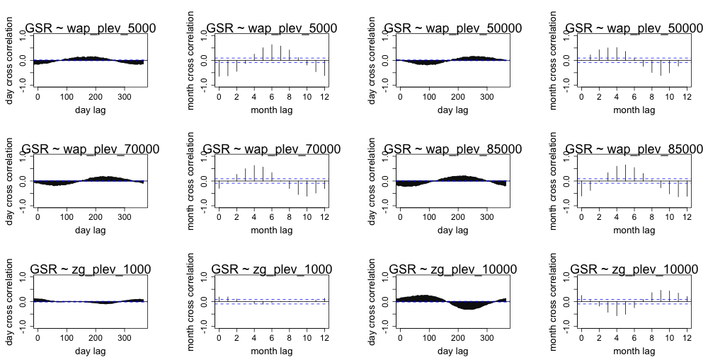
Figure 17 Comparison of daily cross correlation with monthly average cross correlation for each GCM variable against global solar radiation (GSR) at each time scale for the Barmount site.
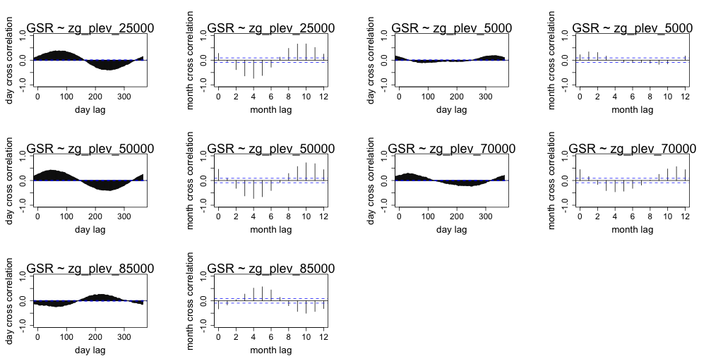
Figure 18 Comparison of daily cross correlation with monthly average cross correlation for each GCM variable against global solar radiation (GSR) at each time scale for the Barmount site.
Data Pre-Processing
The weak correlation between daily covariates and radiation caused issues for building a model that exhibited good connection between predictors and radiation at the daily timescale.
The stronger correlation between month averages of covariates and month averages of radiation enabled a stronger connection. Suggesting the GCM outputs are more connected to seasonal and longer-term trends in the observed global solar radiation, as opposed to daily variation. Daily data was pre-processed to convert GCM outputs and radiation into month averages. Dummy variable columns were added for the month of year (with 11 dummy variables). After processing the resulting GCM variables were lagged over 12 months, so that lags 1 to 12 were added for each variable to each row of the data set.
References

Downscaling Global Climate Models with Convolutional and Long-Short-Term Memory Networks for Solar Energy Applications by C.P. Davey is licensed under a Creative Commons Attribution-NonCommercial-ShareAlike 4.0 International License.