Chapter 4: Model Evaluation and Comparison
Overview
Having trained the CNN-LSTM and baseline models, this chapter is dedicated to the presentation of the evaluation metrics and model comparison. It is structured such that the local (single grid point) models are compared initially with evaluation metrics calculated on the test set between 1989 and 2005, followed by metrics calculated under two future climate change scenarios RCP4.5 and RCP8.5 for the period between 2006 and 2020. Similarly, the same process is applied for the universal downscaling task (9x9 grid) for each of the models.
Local Downscaling Task: Model Evaluation and Comparison
The local downscaling task attempts to synthesise GCM outputs in order to map to observed global solar radiation for a single grid point against station observations. Three kinds of baseline models and two variations of the local CNN-LSTM model, CNN-LSTML and CNN-LSTML DENSE, are constructed for evaluation under this task. Visual model comparison shown in the Taylor diagram below indicates that the CNN-LSTML model has a standard deviation that is closer to that of the observed data however is quite close to the GLM model in terms of standard deviation, correlation and root mean square error (RMSE). The CNN-LSTML DENSE model has a lower RMSE and slightly higher correlation however does not exhibit a standard deviation as close to the observation as the other two models. The GLMNET, GLMNET ALPHA and RF models are quite similar to each other and exhibit similar RMSE, standard deviation and correlation with the observed data.
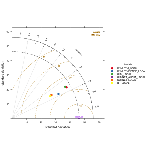
Figure 26 Taylor diagram comparing model prediction for test data from all sites. The models GLM and CNN-LSTML are close in terms of standard deviation of predicted radiation and the correlation with observed global solar radiation. Model CNN-LSTML DENSE is closer in terms of correlation but has slightly more standard deviation in its estimates. RF, GLMNET and GLMNET_ALPHA have similar performance.
There are differences when comparing the performance of each model between sites. In terms of the Kling-Gupta Efficiency (KGE), Table 13 indicates that the CNN-LSTML demonstrates higher efficiency for the majority of sites with the exception of Carpentaria Downs Stations which the same value for KGE between the three models. The CNN-LSTML DENSE model exhibits higher Nash-Sutcliffe Efficiency for 7 of the sites, with the CNN-LSTML model having a higher efficiency index for the remaining sites (Table 14). The CNN-LSTML exhibits higher \(R^{2}\) for all sites except Mossman South Alchera Drive, where the alpha tuned GLMNET has a higher \(R^{2}\) at 0.69 (Table 15). The site with the highest \(R^{2}\) value for the CNN-LSTML model is Springs with a score of 0.85 (or 85% variance explained). A higher Willmott’s Index of Agreement is exhibited by the CNN-LSTML for the majority of sites and is tied with the GLM and CNN-LSTML DENSE models for sites Carpentaria Downs Station and Riverview Hopeland (Table 16). While the GLM exhibits higher agreement for sites Mossman South Alchera Drive and Woolooga and is tied with the CNN-LSTML model for Harewood. In terms of RRMSE both the CNN-LSTM models exhibit lower scores than the other models on all sites, with the CNN-LSTML exhibiting the best value of 7.75% for the Springs site (Table 19). Lower RMSE are achieved by both CNN-LSTM models with the lowest for that model being Woolooga at 20.05\(Wm^{- 2}\) for the CNN-LSTML DENSE model (Table 17). The CNN-LSTML model achieves the lowest RMSE for 8 sites and also has the lowest RMSE overall at the Springs site with an RMSE of 17.78\(Wm^{- 2}\). The largest RMSE for the CNN-LSTML is for the Woolooga site at 26.62\(Wm^{- 2}\). \(CNN - LSTM_{L}\) also produces lower MAE for 8 sites with the lowest MAE being for the Springs observation station with a MAE of 14.05\(Wm^{- 2}\) (Table 18). Lower MAE is exhibited by the CNN-LSTML DENSE model for the remaining sites, like the CNN-LSTML model it exhibits lowest errors for the Springs, Glenlands and Mount Larcom Post Office sites.
Table 13 Kling-Gupta Efficiency comparison per site for each model. Values in bold indicate better scores.
| Model Comparison of Kling-Gupta Efficiency per Site | ||||||
|---|---|---|---|---|---|---|
| Site | CNN-LSTML | CNN-LSTML DENSE | GLM | GLMNET | GLMNET ALPHA | RF |
| Barmount | 0.87 | 0.77 | 0.83 | 0.67 | 0.66 | 0.67 |
| Carpentaria Downs Station | 0.79 | 0.79 | 0.79 | 0.74 | 0.72 | 0.60 |
| Comet Post Office | 0.88 | 0.77 | 0.83 | 0.67 | 0.66 | 0.67 |
| Glenlands | 0.91 | 0.79 | 0.86 | 0.68 | 0.67 | 0.67 |
| Harewood | 0.81 | 0.71 | 0.78 | 0.60 | 0.59 | 0.59 |
| Majors Creek | 0.85 | 0.80 | 0.81 | 0.71 | 0.70 | 0.61 |
| Miles Post Office | 0.82 | 0.71 | 0.78 | 0.60 | 0.59 | 0.60 |
| Mossman South Alchera Drive | 0.82 | 0.82 | 0.79 | 0.76 | 0.74 | 0.55 |
| Mount Larcom Post Office | 0.91 | 0.80 | 0.86 | 0.68 | 0.67 | 0.67 |
| New Caledonia | 0.88 | 0.78 | 0.84 | 0.68 | 0.66 | 0.68 |
| Riverview Hopeland | 0.82 | 0.72 | 0.79 | 0.61 | 0.60 | 0.61 |
| Springs | 0.91 | 0.79 | 0.86 | 0.68 | 0.67 | 0.67 |
| Talagai | 0.87 | 0.77 | 0.83 | 0.67 | 0.66 | 0.67 |
| Woleebee Nevasa | 0.83 | 0.71 | 0.80 | 0.60 | 0.59 | 0.61 |
| Woolooga | 0.87 | 0.78 | 0.87 | 0.67 | 0.65 | 0.66 |
Table 14 Comparison for Nash Sutcliffe Efficiency per site. Values in bold indicate better scores.
| Model Comparison of Nash-Sutcliffe Efficiency per Site | ||||||
|---|---|---|---|---|---|---|
| Site | CNN-LSTML |
CNN-LSTML DENSE |
GLM | GLMNET | GLMNET ALPHA | RF |
| Barmount | 0.76 | 0.75 | 0.65 | 0.66 | 0.67 | 0.65 |
| Carpentaria Downs Station | 0.52 | 0.64 | 0.56 | 0.52 | 0.53 | 0.50 |
| Comet Post Office | 0.75 | 0.74 | 0.69 | 0.65 | 0.66 | 0.65 |
| Glenlands | 0.82 | 0.79 | 0.68 | 0.68 | 0.70 | 0.67 |
| Harewood | 0.75 | 0.78 | 0.77 | 0.70 | 0.69 | 0.70 |
| Majors Creek | 0.69 | 0.73 | 0.62 | 0.62 | 0.64 | 0.56 |
| Miles Post Office | 0.75 | 0.77 | 0.75 | 0.69 | 0.69 | 0.70 |
| Mossman South Alchera Drive | 0.59 | 0.67 | 0.58 | 0.64 | 0.66 | 0.57 |
| Mount Larcom Post Office | 0.83 | 0.81 | 0.71 | 0.71 | 0.72 | 0.70 |
| New Caledonia | 0.77 | 0.75 | 0.70 | 0.66 | 0.67 | 0.67 |
| Riverview Hopeland | 0.75 | 0.79 | 0.77 | 0.71 | 0.70 | 0.72 |
| Springs | 0.84 | 0.82 | 0.73 | 0.72 | 0.73 | 0.71 |
| Talagai | 0.75 | 0.74 | 0.68 | 0.65 | 0.66 | 0.65 |
| Woleebee Nevasa | 0.78 | 0.77 | 0.75 | 0.68 | 0.68 | 0.70 |
| Woolooga | 0.65 | 0.80 | 0.77 | 0.74 | 0.73 | 0.75 |
Table 15 Comparison of \(R^{2}\) for selected sites. Values in bold indicate better scores.
| Model Comparison of \(\mathbf{R}^{\mathbf{2}}\) per Site | ||||||
|---|---|---|---|---|---|---|
| Site | CNN-LSTML | CNN-LSTML DENSE | GLM | GLMNET | GLMNET ALPHA | RF |
| Barmount | 0.77 | 0.76 | 0.69 | 0.72 | 0.72 | 0.70 |
| Carpentaria Downs Station | 0.67 | 0.66 | 0.62 | 0.67 | 0.67 | 0.57 |
| Comet Post Office | 0.77 | 0.75 | 0.71 | 0.71 | 0.71 | 0.71 |
| Glenlands | 0.83 | 0.82 | 0.77 | 0.77 | 0.78 | 0.77 |
| Harewood | 0.83 | 0.82 | 0.79 | 0.78 | 0.78 | 0.80 |
| Majors Creek | 0.74 | 0.73 | 0.67 | 0.70 | 0.70 | 0.63 |
| Miles Post Office | 0.82 | 0.81 | 0.77 | 0.76 | 0.76 | 0.79 |
| Mossman South Alchera Drive | 0.68 | 0.70 | 0.66 | 0.69 | 0.69 | 0.61 |
| Mount Larcom Post Office | 0.84 | 0.83 | 0.76 | 0.79 | 0.79 | 0.79 |
| New Caledonia | 0.78 | 0.77 | 0.72 | 0.73 | 0.73 | 0.73 |
| Riverview Hopeland | 0.83 | 0.82 | 0.78 | 0.78 | 0.78 | 0.81 |
| Springs | 0.85 | 0.84 | 0.78 | 0.80 | 0.80 | 0.80 |
| Talagai | 0.77 | 0.75 | 0.70 | 0.71 | 0.71 | 0.71 |
| Woleebee Nevasa | 0.82 | 0.81 | 0.77 | 0.76 | 0.76 | 0.79 |
| Woolooga | 0.82 | 0.83 | 0.78 | 0.78 | 0.78 | 0.80 |
Table 16 Comparison for Willmott’s index of Agreement. Values in bold indicate better scores.
| Model Comparison of Willmott’s Index of Agreement per Site | ||||||
|---|---|---|---|---|---|---|
| Site | CNN-LSTML | CNN-LSTML DENSE | GLM | GLMNET | GLMNET ALPHA | RF |
| Barmount | 0.94 | 0.92 | 0.91 | 0.88 | 0.88 | 0.88 |
| Carpentaria Downs Station | 0.89 | 0.89 | 0.89 | 0.85 | 0.85 | 0.82 |
| Comet Post Office | 0.93 | 0.92 | 0.91 | 0.88 | 0.88 | 0.88 |
| Glenlands | 0.95 | 0.94 | 0.91 | 0.89 | 0.89 | 0.88 |
| Harewood | 0.93 | 0.92 | 0.93 | 0.88 | 0.88 | 0.88 |
| Majors Creek | 0.92 | 0.92 | 0.90 | 0.87 | 0.88 | 0.84 |
| Miles Post Office | 0.93 | 0.92 | 0.92 | 0.88 | 0.87 | 0.88 |
| Mossman South Alchera Drive | 0.89 | 0.91 | 0.90 | 0.89 | 0.89 | 0.82 |
| Mount Larcom Post Office | 0.96 | 0.94 | 0.92 | 0.90 | 0.90 | 0.89 |
| New Caledonia | 0.94 | 0.92 | 0.92 | 0.88 | 0.88 | 0.88 |
| Riverview Hopeland | 0.93 | 0.93 | 0.93 | 0.88 | 0.88 | 0.89 |
| Springs | 0.96 | 0.94 | 0.93 | 0.90 | 0.90 | 0.90 |
| Talagai | 0.93 | 0.92 | 0.91 | 0.88 | 0.88 | 0.88 |
| Woleebee Nevasa | 0.93 | 0.92 | 0.92 | 0.88 | 0.87 | 0.88 |
| Woolooga | 0.91 | 0.94 | 0.94 | 0.90 | 0.90 | 0.90 |
Table 17 Comparison for RMSE per site. Values in bold indicate better scores.
| Model Comparison of RMSE per Site \(\mathbf{W}\mathbf{m}^{\mathbf{- 2}}\) | ||||||
|---|---|---|---|---|---|---|
| Site | CNN-LSTML | CNN-LSTML DENSE | GLM | GLMNET | GLMNET ALPHA | RF |
| Barmount | 21.50 | 22.22 | 26.34 | 26.15 | 25.77 | 26.45 |
| Carpentaria Downs Station | 26.45 | 23.13 | 25.72 | 26.82 | 26.36 | 27.20 |
| Comet Post Office | 21.77 | 22.51 | 24.94 | 26.46 | 26.06 | 26.19 |
| Glenlands | 18.46 | 20.00 | 25.21 | 25.12 | 24.40 | 25.53 |
| Harewood | 25.19 | 23.81 | 24.41 | 28.16 | 28.25 | 27.83 |
| Majors Creek | 22.73 | 21.25 | 25.49 | 25.49 | 24.69 | 27.29 |
| Miles Post Office | 25.28 | 24.10 | 25.65 | 28.28 | 28.37 | 27.68 |
| Mossman South Alchera Drive | 24.27 | 21.67 | 24.81 | 22.99 | 22.20 | 25.21 |
| Mount Larcom Post Office | 18.04 | 19.38 | 23.97 | 24.26 | 23.77 | 24.65 |
| New Caledonia | 20.95 | 21.77 | 24.24 | 25.84 | 25.47 | 25.58 |
| Riverview Hopeland | 25.18 | 23.11 | 24.42 | 27.36 | 27.50 | 26.66 |
| Springs | 17.78 | 19.02 | 23.34 | 24.03 | 23.60 | 24.35 |
| Talagai | 21.81 | 22.51 | 25.07 | 26.36 | 25.99 | 26.30 |
| Woleebee Nevasa | 23.59 | 24.08 | 25.21 | 28.39 | 28.40 | 27.66 |
| Woolooga | 26.62 | 20.05 | 21.79 | 23.28 | 23.82 | 23.04 |
Table 18 Comparison of MAE per site. Values in bold indicate better scores.
| Model Comparison of MAE per Site \(\mathbf{W}\mathbf{m}^{\mathbf{- 2}}\) | ||||||
|---|---|---|---|---|---|---|
| Site | CNN-LSTML | CNN-LSTML DENSE | GLM | GLMNET | GLMNET ALPHA | RF |
| Barmount | 16.80 | 16.82 | 21.58 | 20.65 | 20.26 | 20.65 |
| Carpentaria Downs Station | 22.11 | 18.30 | 19.33 | 22.35 | 21.69 | 21.42 |
| Comet Post Office | 16.93 | 17.16 | 20.23 | 20.66 | 20.30 | 20.19 |
| Glenlands | 14.54 | 15.13 | 20.64 | 19.43 | 18.88 | 20.00 |
| Harewood | 19.78 | 18.85 | 19.52 | 22.63 | 22.81 | 22.92 |
| Majors Creek | 17.56 | 16.06 | 19.20 | 20.44 | 19.58 | 21.56 |
| Miles Post Office | 19.66 | 19.09 | 20.67 | 22.71 | 22.85 | 22.61 |
| Mossman South Alchera Drive | 19.67 | 15.95 | 19.13 | 18.59 | 17.73 | 20.40 |
| Mount Larcom Post Office | 14.37 | 14.77 | 19.59 | 18.63 | 18.33 | 19.54 |
| New Caledonia | 16.34 | 16.58 | 19.77 | 20.14 | 19.76 | 19.83 |
| Riverview Hopeland | 19.70 | 18.26 | 19.57 | 21.94 | 22.23 | 21.84 |
| Springs | 14.05 | 14.70 | 18.93 | 18.42 | 18.28 | 19.56 |
| Talagai | 16.73 | 17.06 | 20.36 | 20.67 | 20.29 | 20.32 |
| Woleebee Nevasa | 18.10 | 19.04 | 20.21 | 22.73 | 22.80 | 22.37 |
| Woolooga | 21.01 | 15.88 | 17.93 | 18.84 | 19.48 | 19.02 |
Table 19 Comparison of RRMSE per site. Values in bold indicate better scores.
| Model Comparison of RRMSE per Site % | ||||||
|---|---|---|---|---|---|---|
| Site | CNN-LSTML | CNN-LSTML DENSE | GLM | GLMNET | GLMNET ALPHA | RF |
| Barmount | 9.37 | 9.69 | 11.47 | 11.39 | 11.22 | 11.52 |
| Carpentaria Downs Station | 11.30 | 9.88 | 10.96 | 11.43 | 11.23 | 11.59 |
| Comet Post Office | 9.44 | 9.76 | 10.80 | 11.45 | 11.28 | 11.33 |
| Glenlands | 7.96 | 8.63 | 10.87 | 10.83 | 10.52 | 11.01 |
| Harewood | 11.09 | 10.48 | 10.75 | 12.40 | 12.44 | 12.26 |
| Majors Creek | 9.82 | 9.18 | 11.00 | 11.00 | 10.66 | 11.77 |
| Miles Post Office | 11.13 | 10.61 | 11.29 | 12.45 | 12.49 | 12.19 |
| Mossman South Alchera Drive | 10.76 | 9.60 | 10.97 | 10.16 | 9.81 | 11.14 |
| Mount Larcom Post Office | 7.85 | 8.43 | 10.41 | 10.54 | 10.32 | 10.71 |
| New Caledonia | 9.08 | 9.44 | 10.50 | 11.19 | 11.03 | 11.08 |
| Riverview Hopeland | 11.14 | 10.22 | 10.81 | 12.11 | 12.17 | 11.80 |
| Springs | 7.75 | 8.29 | 10.15 | 10.45 | 10.27 | 10.59 |
| Talagai | 9.46 | 9.76 | 10.86 | 11.42 | 11.26 | 11.39 |
| Woleebee Nevasa | 10.33 | 10.55 | 11.04 | 12.44 | 12.44 | 12.12 |
| Woolooga | 12.22 | 9.20 | 9.99 | 10.67 | 10.92 | 10.56 |
There are performance differences in each model between different sites, with the CNN-LSTML, CNN-LSTML DENSE and GLM models exhibiting best generalisation capabilities between sites. Locations where the CNN-LSTML model performs best include Springs and Mount Larcom Post Office, while on the other extreme, the model has lower performance metrics for the sites Carpentaria Downs Station and Woolooga where the CNN-LSTML and GLM models exhibits good performance. Comparison of both extremes is useful in order to further review the bias of the models.
The scatter plot of observations against predictions at the Springs site (Figure 27) illustrates a tendency of the models to underestimate the radiation at the Springs site in the upper extremes and a tendency to overestimate in the lower range. Whereas both GLM and CNN-LSTM models appear to have similar levels of positive and negative residuals. The CNN-LSTML DENSE model appears to have a less uniform estimation for radiation with values clustered between 160 to 180 \(Wm^{- 2}\), 200 to 220\(\text{W}m^{- 2}\) and between 240 and 280 \(Wm^{- 2}\).
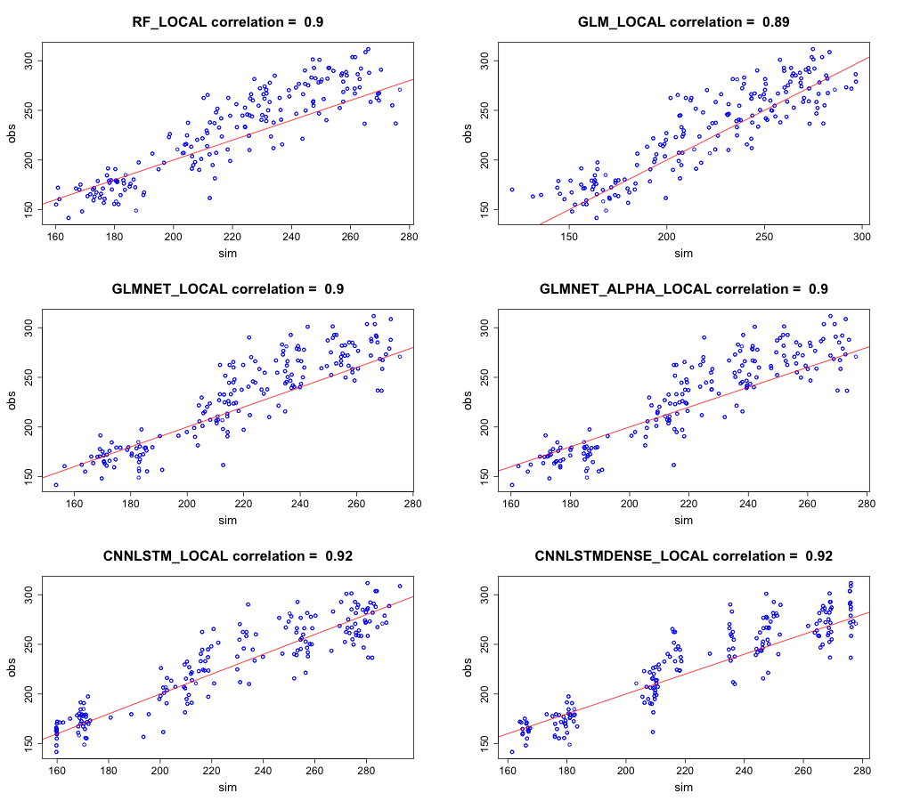
Figure 27 Correlation of simulated radiation versus observed global solar radiation for the site Springs for all models.
The bias in residuals is more evident in the error histogram for the site shown in Figure 28. There is a slight right-hand side skew visible in the CNN-LSTML DENSE model and to a lesser extent for the CNN-LSTML model. The GLM model appears to have a less normal distribution for the residuals in comparison to the CNN-LSTML model.
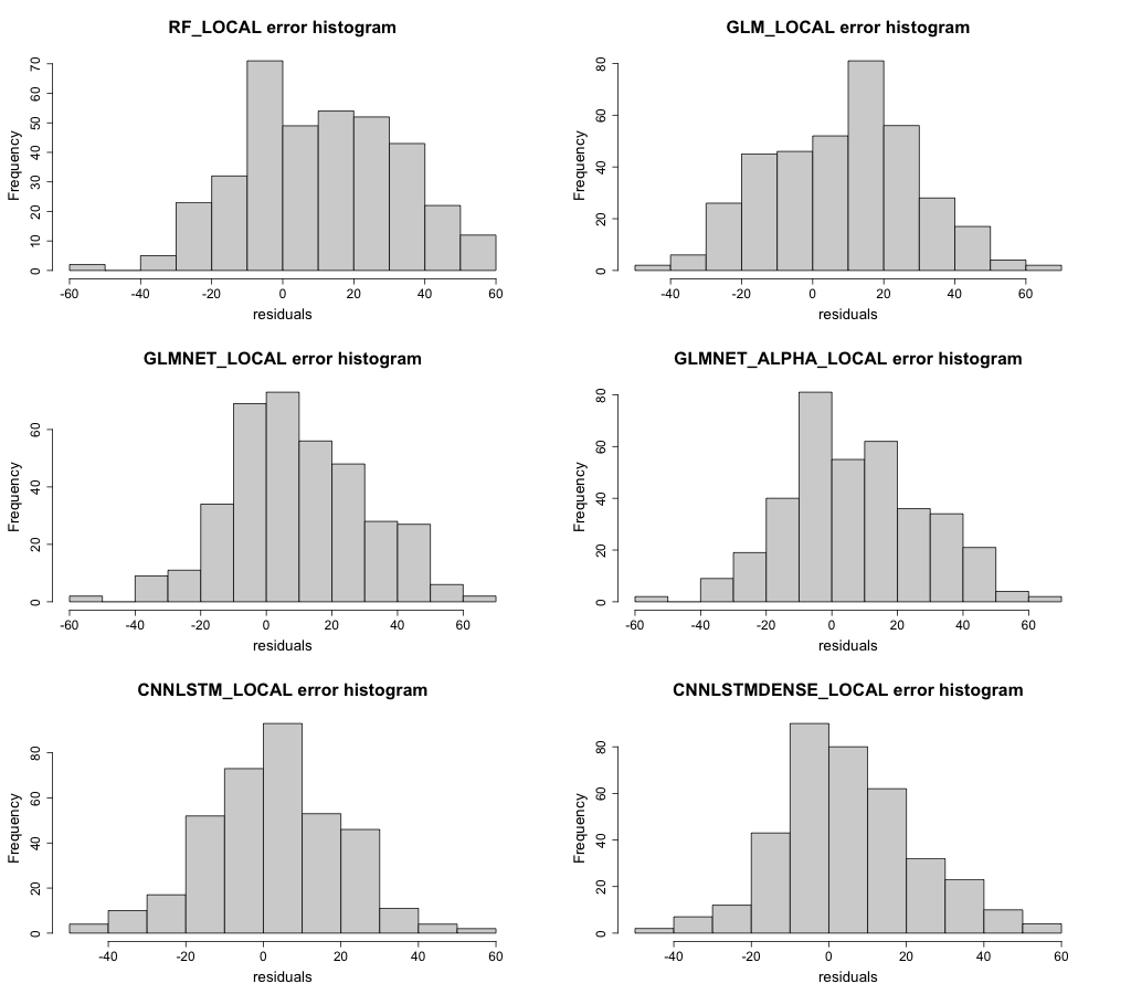
Figure 28 Histogram of residuals for all models at site Springs.
Correlation between observed and simulated radiation for each model at the Carpentaria Downs Station is shown in Figure 29. The CNN-LSTML model exhibits a number of outliers which overestimate radiation at this site (values below the regression line) with lower prediction values tending to underestimate radiation. This is a trait shared with the other models, although the GLM model appears to have a higher density closer to 0 with a number of outliers in the lower range of predicted values tending to under-estimate the radiation. Smaller values for residuals are also visible in the histograms in Figure 30, where there is a left-hand skew for negative residuals for the CNN-LSTML model (and other models).
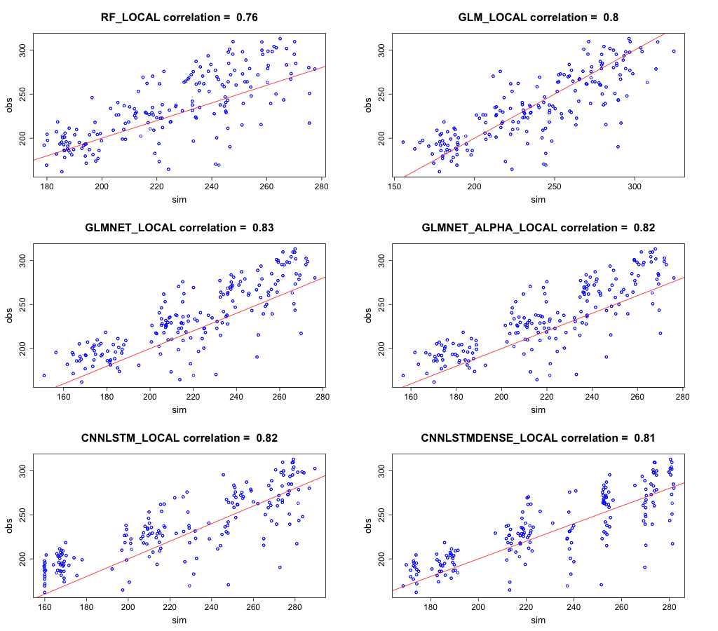
Figure 29 Observed global solar radiation versus simulated radiation for site Carpentaria Downs Station.
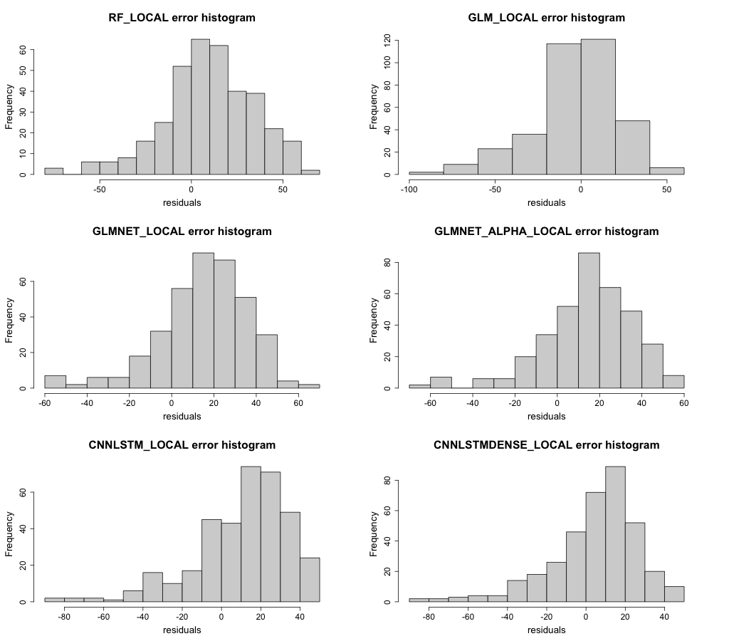
Figure 30 Histogram of residuals for each model at the Carpentaria Downs Station.
The GLM and both CNN-LSTM models have similar generalisation capabilities with both of the CNN-LSTM models exhibiting better performance across most sites. The two sites illustrated represent the extremes between best and worst performance for the CNN-LSTML model. The timeseries plot for the Springs site indicates the other models are less capable of capturing the extremes of the radiation signal at that site, with the magnitude of estimates having less extreme peaks (Figure 31). The GLM model underestimates the lower peaks in radiation with one outlier near 2005. The CNN-LSTML model provides a good approximation of radiation at the site and the CNN-LSTML DENSE model appears not to estimate the extremes quite as well as its peer.
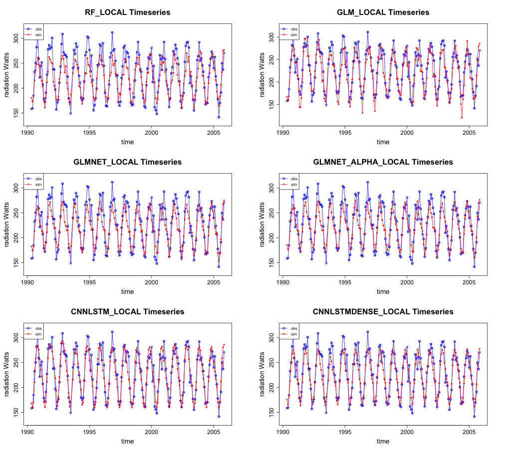
Figure 31 Timeseries of the test set observed versus simulated radiation for each model at site Springs.
The worst-case site for the CNN-LSTML model, Carpentaria Downs Station, is shown in Figure 32. In this case the underestimation for radiation is visible for the CNN-LSTML model. The other models appear to underestimate the peaks and troughs significantly, indicating that both the GLM and CNN-LSTML DENSE models appear to have a better ability to estimate the extremes.
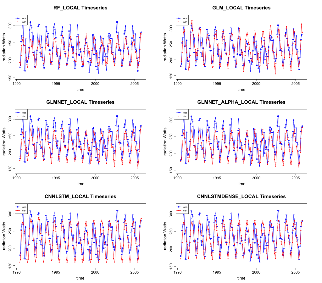
Figure 32 Timeseries of test set observations and simulated radiation for site Carpentaria Downs Station.
Examining mean error per month for the three models (GLM, CNN-LSTML and CNN-LSTML DENSE), at the Springs site indicates that the GLM has highest errors in January, February, and March, with a range between 2.32\(Wm^{- 2}\) in April and 24.75\(\text{W}m^{- 2}\) in March (Figure 33). The CNN-LSTM exhibits largest mean error in January, February and March with a range between -8.36\(\text{W}m^{- 2}\) in October and 19.66\(\text{W}m^{- 2}\) in March (Figure 34). Similar to the CNN-LSTML model, the CNN-LSTML DENSE has largest mean error for Springs in months of January, February and March with a range between -5.84\(\text{W}m^{- 2}\ \)in May to 24.39\(\text{W}m^{- 2}\) in March (Figure 35). For Carpentaria Downs Station, the GLM is indicated to have largest mean error in January, February and December, with a range between -29.61\(\text{W}m^{- 2}\) in December and 8.18\(\text{W}m^{- 2}\) in August (Figure 36). Larger average error for the CNN-LSTML model at the same site occur in July and have a range between -15.19\(\text{W}m^{- 2}\) in December and 30.42 \(Wm^{- 2}\) in July. The CNN-LSTML DENSE model also exhibits largest average error in September in Figure 38, having a range between -14.18\(\text{W}m^{- 2}\) in February to 18.14\(\text{W}m^{- 2}\) in September.
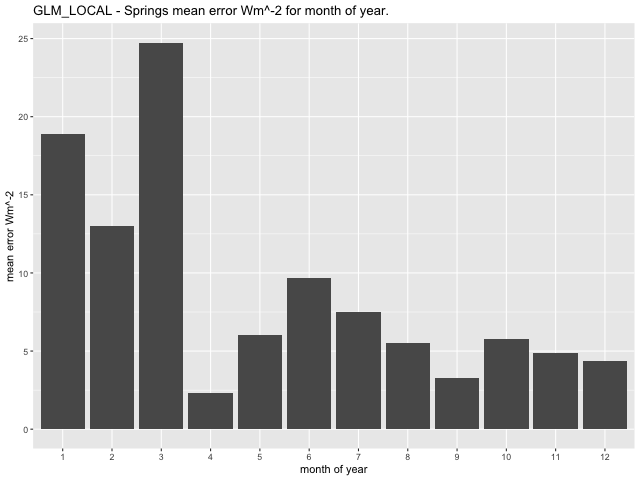
Figure 33 GLM model mean error per month at the Springs site.
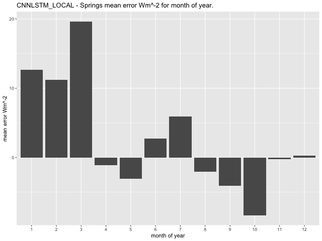
Figure 34 CNN-LSTML model mean error per month for the Springs site.
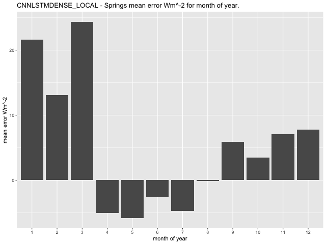
Figure 35 CNN-LSTML DENSE mean error per month for the Springs site.
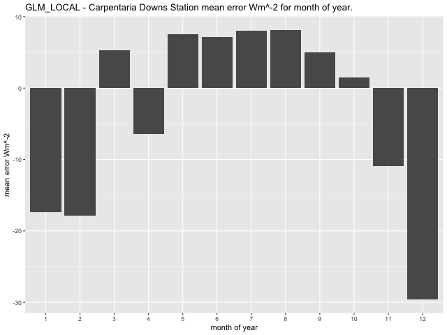
Figure 36 GLM model mean error per month for Carpentaria Downs Station.
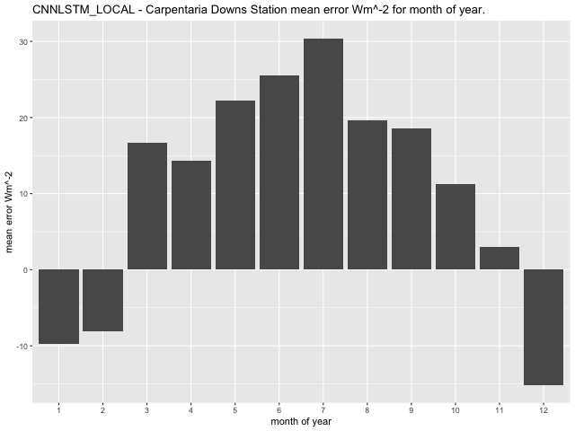
Figure 37 CNN-LSTML model mean error per month for Carpentaria Downs Station.
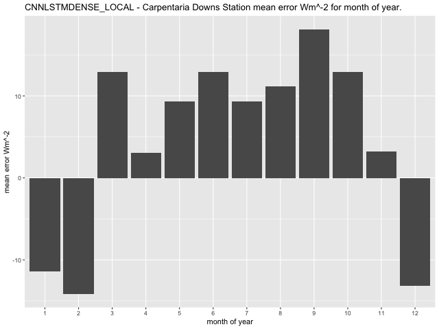
Figure 38 CNN-LSTML DENSE model mean error per month for Carpentaria Downs Station.
Future Scenario RCP4.5 2006 to 2020
The metrics for each site produced by the evaluation of each model are listed in Table 20. The CNN-LSTML model demonstrates higher \(R^{2}\) in the evaluation metrics under the RCP4.5 profile for the period 2006 to 2020. The CNN-LSTML model exhibits good performance second to the CNN-LSTML DENSE model which achieves better values for the other metrics for most sites. However as indicated in the quantile regression for the bias the CNN-LSTML DENSE model exhibits higher non-uniform variance than the other models. The GLM model achieves a higher \(R^{2}\) for Majors Creek but exhibits a negative efficiency for the same site and several of the other sites.
Table 20 Evaluation metrics for each module under the RCP4.5 projection. Kling-Gupta Efficiency (KGE), Nash-Sutcliffe Efficiency (Ez), Coefficient of determination \(R^{2}\), Willmott’s Index of Agreement d, Root Mean Square Error RMSE, Mean Absolute Error (MAE) and Relative Root Mean Square Error (RRMSE). Values in bold indicate better scores.
| Site Name | Model Name | KGE | E | \[\mathbf{R}^{\mathbf{2}}\] | d | RMSE \(\mathbf{W}\mathbf{m}^{\mathbf{- 2}}\) | MAE \(\mathbf{W}\mathbf{m}^{\mathbf{- 2}}\) | RRMSE % |
|---|---|---|---|---|---|---|---|---|
| Barmount | CNN-LSTML | 0.88 | 0.67 | 0.84 | 0.92 | 24.45 | 19.83 | 11.53 |
| CNN-LSTML DENSE | 0.86 | 0.74 | 0.84 | 0.93 | 21.81 | 17.95 | 10.28 | |
| GLM | 0.74 | -0.25 | 0.76 | 0.77 | 49.33 | 43.14 | 23.34 | |
| Carpentaria Downs Station | CNN-LSTML | 0.80 | 0.68 | 0.77 | 0.93 | 21.20 | 17.54 | 9.45 |
| CNN-LSTML DENSE | 0.88 | 0.75 | 0.77 | 0.94 | 18.53 | 15.46 | 8.26 | |
| GLM | 0.73 | -0.08 | 0.80 | 0.80 | 39.83 | 34.65 | 17.68 | |
| Comet Post Office | CNN-LSTML | 0.91 | 0.77 | 0.88 | 0.94 | 20.75 | 17.24 | 9.50 |
| CNN-LSTML DENSE | 0.86 | 0.83 | 0.86 | 0.95 | 17.74 | 14.89 | 8.13 | |
| GLM | 0.78 | 0.00 | 0.78 | 0.80 | 45.45 | 39.58 | 20.94 | |
| Glenlands | CNN-LSTML | 0.86 | 0.56 | 0.84 | 0.90 | 28.24 | 23.48 | 13.49 |
| CNN-LSTML DENSE | 0.86 | 0.69 | 0.83 | 0.91 | 23.67 | 19.29 | 11.30 | |
| GLM | 0.75 | -0.14 | 0.77 | 0.78 | 47.08 | 40.87 | 22.46 | |
| Harewood | CNN-LSTML | 0.82 | 0.69 | 0.85 | 0.91 | 27.69 | 23.56 | 12.76 |
| CNN-LSTML DENSE | 0.77 | 0.77 | 0.82 | 0.92 | 24.02 | 18.89 | 11.07 | |
| GLM | 0.78 | 0.16 | 0.80 | 0.82 | 47.06 | 41.61 | 21.91 | |
| Majors Creek | CNN-LSTML | 0.80 | 0.47 | 0.73 | 0.88 | 28.31 | 20.84 | 13.32 |
| CNN-LSTML DENSE | 0.84 | 0.61 | 0.73 | 0.90 | 24.21 | 18.37 | 11.39 | |
| GLM | 0.70 | -0.44 | 0.76 | 0.76 | 48.27 | 42.26 | 22.56 | |
| Miles Post Office | CNN-LSTML | 0.83 | 0.71 | 0.86 | 0.92 | 26.42 | 22.46 | 12.12 |
| CNN-LSTML DENSE | 0.77 | 0.78 | 0.82 | 0.93 | 23.15 | 18.03 | 10.62 | |
| GLM | 0.79 | 0.22 | 0.79 | 0.83 | 45.25 | 39.42 | 20.97 | |
| Mossman South Alchera Drive | CNN-LSTML | 0.80 | 0.44 | 0.69 | 0.87 | 29.98 | 22.52 | 14.60 |
| CNN-LSTML DENSE | 0.78 | 0.42 | 0.68 | 0.85 | 30.56 | 23.83 | 14.88 | |
| GLM | 0.70 | -0.34 | 0.64 | 0.75 | 47.75 | 39.72 | 22.85 | |
| Mount Larcom Post Office | CNN-LSTML | 0.88 | 0.67 | 0.85 | 0.92 | 24.68 | 20.45 | 11.69 |
| CNN-LSTML DENSE | 0.86 | 0.73 | 0.84 | 0.92 | 22.40 | 18.80 | 10.61 | |
| GLM | 0.75 | -0.17 | 0.77 | 0.78 | 48.19 | 42.40 | 22.88 | |
| New Caledonia | CNN-LSTML | 0.90 | 0.72 | 0.87 | 0.93 | 22.94 | 18.93 | 10.63 |
| CNN-LSTML DENSE | 0.86 | 0.80 | 0.85 | 0.94 | 19.29 | 16.08 | 8.94 | |
| GLM | 0.77 | -0.10 | 0.78 | 0.78 | 47.51 | 41.76 | 22.12 | |
| Riverview Hopeland | CNN-LSTML | 0.82 | 0.67 | 0.85 | 0.91 | 28.36 | 24.28 | 13.13 |
| CNN-LSTML DENSE | 0.77 | 0.76 | 0.81 | 0.92 | 24.29 | 19.30 | 11.25 | |
| GLM | 0.78 | 0.15 | 0.79 | 0.81 | 46.93 | 41.13 | 21.95 | |
| Springs | CNN-LSTML | 0.88 | 0.66 | 0.84 | 0.92 | 24.95 | 20.94 | 11.82 |
| CNN-LSTML DENSE | 0.87 | 0.72 | 0.83 | 0.92 | 22.59 | 19.29 | 10.70 | |
| GLM | 0.75 | -0.20 | 0.78 | 0.77 | 47.94 | 42.45 | 22.76 | |
| Talagai | CNN-LSTML | 0.90 | 0.75 | 0.87 | 0.94 | 21.51 | 17.60 | 9.90 |
| CNN-LSTML DENSE | 0.87 | 0.82 | 0.86 | 0.95 | 18.03 | 14.99 | 8.29 | |
| GLM | 0.78 | -0.04 | 0.78 | 0.79 | 46.15 | 40.44 | 21.36 | |
| Woleebee Nevasa | CNN-LSTML | 0.84 | 0.73 | 0.86 | 0.92 | 25.36 | 21.46 | 11.58 |
| CNN-LSTML DENSE | 0.78 | 0.79 | 0.82 | 0.93 | 22.40 | 17.30 | 10.23 | |
| GLM | 0.79 | 0.18 | 0.78 | 0.82 | 45.90 | 39.94 | 21.17 | |
| Woolooga | CNN-LSTML | 0.84 | 0.52 | 0.81 | 0.88 | 31.93 | 27.21 | 15.22 |
| CNN-LSTML DENSE | 0.81 | 0.67 | 0.79 | 0.90 | 26.47 | 22.07 | 12.61 | |
| GLM | 0.78 | 0.05 | 0.79 | 0.81 | 45.40 | 39.83 | 21.78 |
The most accurate metrics for the CNN-LSTML and CNN-LSTML DENSE models are associated with Comet Post Office under the RCP4.5 profile. The timeseries plot for this site for each model is shown in Figure 39. The GLM model appears to over-estimate the radiation at this site and does not estimate the extremes as well as the other models. The CNN-LSTML DENSE appears to capture the time series well for this site. However, does not appear to capture the extremes as well as the CNN-LSTML model.
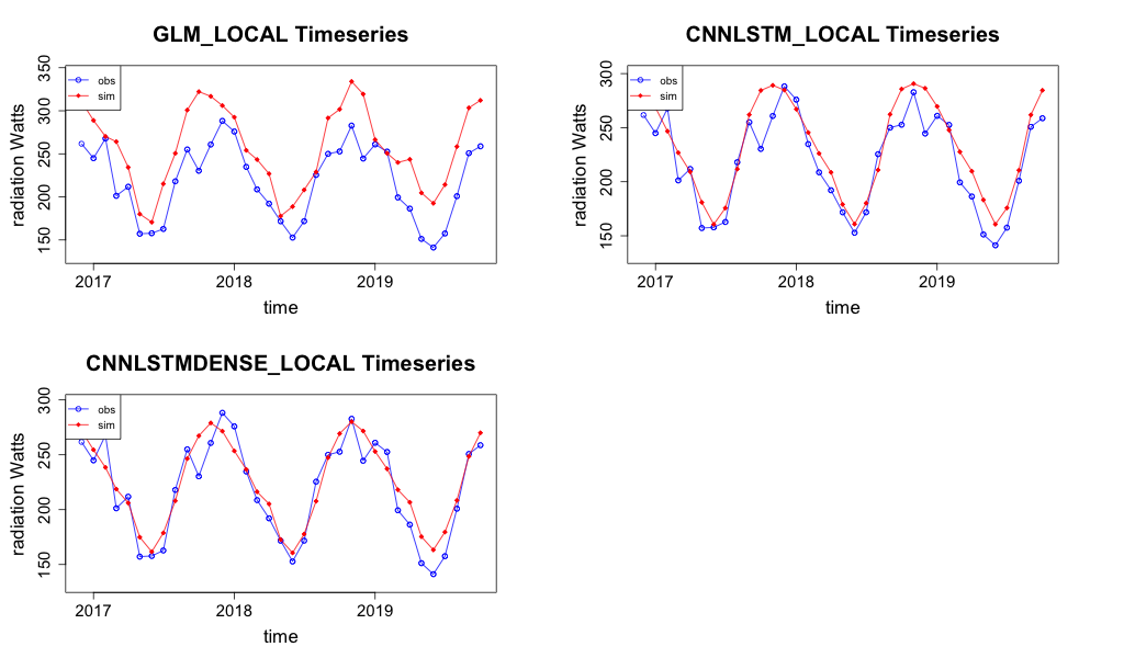
Figure 39 Projection of radiation for both models between 2016 and 2020 under the RCP4.5 climate warming scenario for the Comet Post Office observation station.
Majors Creek exhibited higher \(R^{2}\) for the GLM model, this site is selected as the worst performing site under the RCP4.5 projection for 2006 to 2020 period for the CNN-LSTML and CNN-LSTML DENSE model. The timeseries for each model at this site are shown in Figure 40.
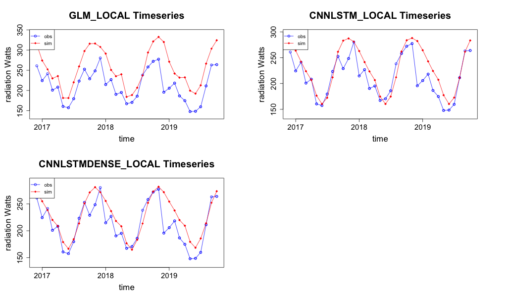
Figure 40 Prediction of radiation timeseries for both models under the
RCP4.5 climate warming scenario at the Majors Creek observation site.The both the CNN-LSTML and CNN-LSTML DENSE models estimate the extremes more effectively at this site than the GLM model. The estimate appears to be smooth missing some of the variability in the average radiation per month.
Average mean error per month of year for the GLM model at the Comet Post Office site has the range between -64.69\(Wm^{- 2}\) in October and -6.58\(\text{W}m^{- 2}\) in February (Figure 41). The CNN-LSTML model exhibits a maximum average error per month in October having a range between -37.6\(\text{W}m^{- 2}\) in October and 5.06\(\text{W}m^{- 2}\) in February (Figure 42). Similarly the CNN-LSTML DENSE model has a largest average error in October of -21.58\(\text{W}m^{- 2}\) ranging to 6.91\(\text{W}m^{- 2}\) in January (Figure 43).
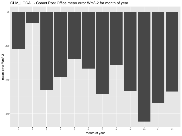
Figure 41 GLM model average RCP4.5 prediction error per month of year 2006-2020 for the Comet Post Office Site.
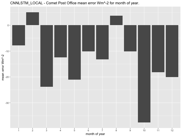
Figure 42 CNN-LSTML model average RCP4.5 prediction error per month of year 2006-2020 for the Comet Post Office Site.
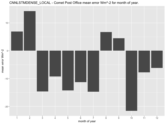
Figure 43 CNN-LSTML DENSE model average RCP4.5 prediction error per month of year 2006-2020 for the Comet Post Office Site.
Future Scenario RCP8.5 2006 to 2020
The evaluation metrics for both models under the RCP8.5 climate warming scenario for the period 2006-2020 are listed in Table 21. The GLM model shows an improvement in metric evaluation under the RCP8.5 climate warming scenario, however in most cases with the exception of the Majors Creek observation site, does not perform as well as the CNN-LSTML and CNN-LSTML DENSE models in evaluation. For the majority of sites, the CNN-LSTML DENSE produces better metrics in comparison to CNN-LSTML.
Table 21 Evaluation metrics for each model under the RCP8.5 climate warming scenario between 2006 - 2020. Values in bold indicate better scores.
| Site Name | Model Name | KGE | E | \[\mathbf{R}^{\mathbf{2}}\] | d | RMSE \(\mathbf{W}\mathbf{m}^{\mathbf{- 2}}\) | MAE \(\mathbf{W}\mathbf{m}^{\mathbf{- 2}}\) | RRMSE % |
|---|---|---|---|---|---|---|---|---|
| Barmount | CNN-LSTML | 0.89 | 0.72 | 0.85 | 0.93 | 22.53 | 17.98 | 10.62 |
| CNN-LSTML DENSE | 0.86 | 0.80 | 0.85 | 0.94 | 19.29 | 15.70 | 9.09 | |
| GLM | 0.76 | 0.44 | 0.77 | 0.89 | 32.97 | 27.35 | 15.60 | |
| Carpentaria Downs Station | CNN-LSTML | 0.82 | 0.71 | 0.78 | 0.93 | 20.03 | 16.66 | 8.93 |
| CNN-LSTML DENSE | 0.88 | 0.77 | 0.78 | 0.94 | 18.03 | 14.87 | 8.03 | |
| GLM | 0.67 | 0.19 | 0.77 | 0.85 | 34.44 | 28.62 | 15.29 | |
| Comet Post Office | CNN-LSTML | 0.92 | 0.81 | 0.88 | 0.95 | 18.97 | 15.52 | 8.69 |
| CNN-LSTML DENSE | 0.87 | 0.87 | 0.88 | 0.96 | 15.41 | 12.97 | 7.06 | |
| GLM | 0.80 | 0.43 | 0.79 | 0.88 | 34.29 | 28.99 | 15.80 | |
| Glenlands | CNN-LSTML | 0.87 | 0.62 | 0.85 | 0.91 | 26.32 | 21.45 | 12.57 |
| CNN-LSTML DENSE | 0.86 | 0.76 | 0.85 | 0.93 | 20.71 | 16.55 | 9.89 | |
| GLM | 0.77 | 0.40 | 0.75 | 0.88 | 33.98 | 28.01 | 16.21 | |
| Harewood | CNN-LSTML | 0.84 | 0.75 | 0.85 | 0.93 | 24.95 | 20.88 | 11.49 |
| CNN-LSTML DENSE | 0.76 | 0.83 | 0.86 | 0.94 | 20.67 | 15.55 | 9.52 | |
| GLM | 0.81 | 0.45 | 0.81 | 0.88 | 38.21 | 33.19 | 17.79 | |
| Majors Creek | CNN-LSTML | 0.81 | 0.54 | 0.74 | 0.90 | 26.38 | 19.29 | 12.41 |
| CNN-LSTML DENSE | 0.84 | 0.63 | 0.74 | 0.90 | 23.58 | 17.49 | 11.09 | |
| GLM | 0.69 | 0.35 | 0.75 | 0.88 | 32.43 | 27.23 | 15.16 | |
| Miles Post Office | CNN-LSTML | 0.85 | 0.77 | 0.85 | 0.93 | 23.80 | 19.89 | 10.91 |
| CNN-LSTML DENSE | 0.77 | 0.83 | 0.86 | 0.95 | 20.02 | 14.88 | 9.18 | |
| GLM | 0.79 | 0.37 | 0.80 | 0.87 | 40.49 | 34.99 | 18.76 | |
| Mossman South Alchera Drive | CNN-LSTML | 0.82 | 0.57 | 0.70 | 0.89 | 26.17 | 20.31 | 12.74 |
| CNN-LSTML DENSE | 0.79 | 0.43 | 0.68 | 0.85 | 30.22 | 23.45 | 14.71 | |
| GLM | 0.68 | 0.16 | 0.59 | 0.83 | 37.84 | 31.37 | 18.11 | |
| Mount Larcom Post Office | CNN-LSTML | 0.89 | 0.72 | 0.85 | 0.93 | 22.81 | 18.72 | 10.81 |
| CNN-LSTML DENSE | 0.86 | 0.81 | 0.86 | 0.94 | 19.03 | 15.72 | 9.01 | |
| GLM | 0.80 | 0.46 | 0.77 | 0.88 | 32.69 | 26.70 | 15.52 | |
| New Caledonia | CNN-LSTML | 0.91 | 0.77 | 0.87 | 0.94 | 21.01 | 17.04 | 9.74 |
| CNN-LSTML DENSE | 0.86 | 0.85 | 0.88 | 0.96 | 16.73 | 14.01 | 7.75 | |
| GLM | 0.80 | 0.48 | 0.79 | 0.89 | 32.74 | 27.36 | 15.24 | |
| Riverview Hopeland | CNN-LSTML | 0.84 | 0.73 | 0.84 | 0.92 | 25.55 | 21.54 | 11.83 |
| CNN-LSTML DENSE | 0.76 | 0.82 | 0.85 | 0.94 | 20.86 | 15.95 | 9.66 | |
| GLM | 0.80 | 0.41 | 0.79 | 0.88 | 38.97 | 33.50 | 18.23 | |
| Springs | CNN-LSTML | 0.89 | 0.71 | 0.84 | 0.93 | 23.12 | 19.23 | 10.96 |
| CNN-LSTML DENSE | 0.87 | 0.80 | 0.86 | 0.94 | 19.13 | 16.04 | 9.06 | |
| GLM | 0.79 | 0.44 | 0.76 | 0.88 | 32.81 | 26.94 | 15.57 | |
| Talagai | CNN-LSTML | 0.91 | 0.79 | 0.88 | 0.95 | 19.61 | 15.74 | 9.02 |
| CNN-LSTML DENSE | 0.87 | 0.87 | 0.88 | 0.96 | 15.70 | 13.06 | 7.22 | |
| GLM | 0.80 | 0.45 | 0.79 | 0.89 | 33.36 | 28.13 | 15.44 | |
| Woleebee Nevasa | CNN-LSTML | 0.86 | 0.78 | 0.85 | 0.94 | 22.84 | 18.87 | 10.43 |
| CNN-LSTML DENSE | 0.77 | 0.84 | 0.86 | 0.95 | 19.50 | 14.45 | 8.90 | |
| GLM | 0.78 | 0.36 | 0.80 | 0.87 | 40.69 | 34.97 | 18.76 | |
| Woolooga | CNN-LSTML | 0.85 | 0.59 | 0.81 | 0.90 | 29.38 | 24.50 | 14.00 |
| CNN-LSTML DENSE | 0.80 | 0.76 | 0.82 | 0.93 | 22.51 | 18.59 | 10.73 | |
| GLM | 0.77 | 0.35 | 0.78 | 0.87 | 37.53 | 32.51 | 18.00 | |
Comet Post Office again appears to be estimated well by the CNN-LSTML model under the RCP8.5 profile. The time series prediction at this site is shown in Figure 44.
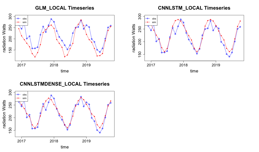
Figure 44 Prediction of Radiation for both models under the RCP8.5 climate warming scenario for the period 2016 to 2020 at Comet Post Office.
The GLM model achieved a higher \(R^{2}\) and lower peak percentage deviation than the CNN-LSTML model for the Majors Creek observation site. The timeseries projection for this site is shown in Figure 45. The GLM model appears to consistently underestimate the radiation for this site, whereas the timeseries for both CNN-LSTM models appears to over estimate the lower extremes of radiation and under estimate the upper extremes. These models also produce a smooth estimate of the radiation, appearing to provide a good representation of the seasonality in the data rather than for the individual monthly variation. The CNN-LSTML appears to tolerate the shift in covariates between profiles and matches the seasonal change of the radiation well for each projection.
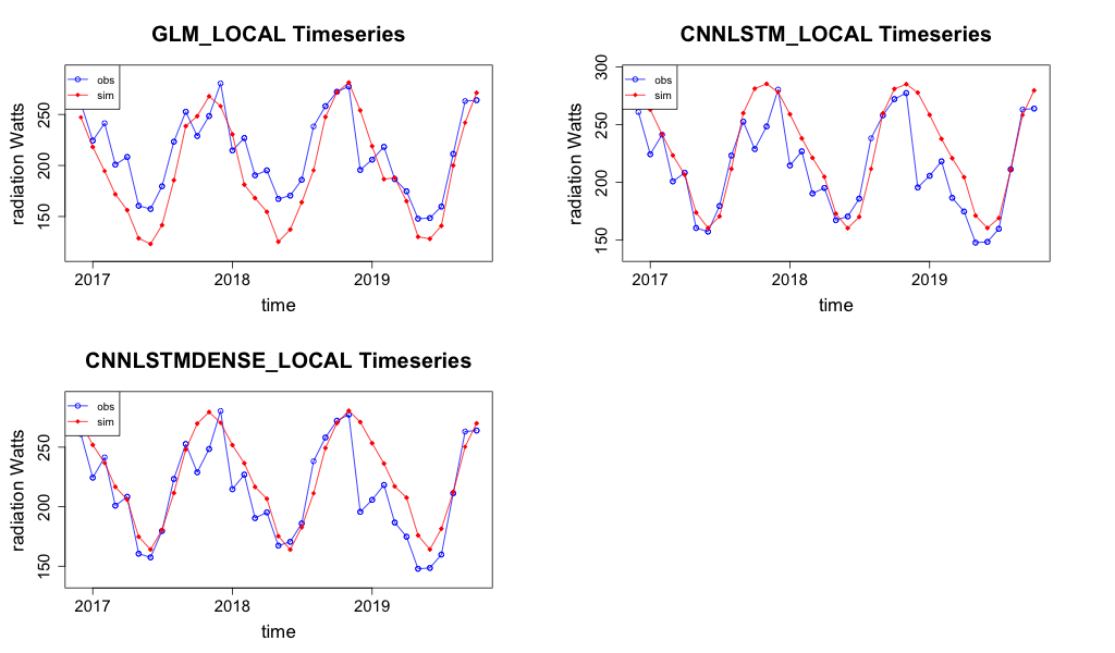
Figure 45 Prediction of radiation for Majors Creek observation site under the RCP8.5 climate warming scenario between 2016 and 2020 for both models.
At the Comet Post Office observation station, the GLM model exhibits the highest average error in February for RCP8.5 scenario, with a range between 55.31\(Wm^{- 2}\) in February and -6.22\(Wm^{- 2}\) in October (Figure 46). The CNN-LSTML model has a larger average error in October under the RCP8.5 profile (similar to RCP4.5) with a range between -35.48\(\text{W}m^{- 2}\) in October and 8.44\(\text{W}m^{- 2}\) in February (Figure 47). The CNN-LSTML DENSE also exhibits the largest average error during October with a range between -19.15\(\text{W}m^{- 2}\) to 15.65\(\text{W}m^{- 2}\) (Figure 48).
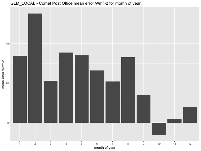
Figure 46 GLM model average RCP8.5 prediction error per month of year 2006-2020 for the Comet Post Office Site.
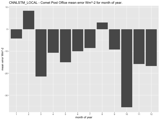
Figure 47 CNN-LSTML model average RCP8.5 prediction error per month of year 2006-2020 for the Comet Post Office Site.
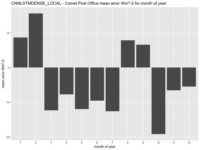
Figure 48 CNN-LSTML DENSE model average RCP8.5 prediction error per month of year 2006-2020 for the Comet Post Office Site.

Downscaling Global Climate Models with Convolutional and Long-Short-Term Memory Networks for Solar Energy Applications by C.P. Davey is licensed under a Creative Commons Attribution-NonCommercial-ShareAlike 4.0 International License.