Chapter 3: Model Development
Model Development
The approach taken in the development of the CNN-LSTM is to first leverage a grid search in determining the set of parameterisations to choose for the configuration of the network modules for subsequent training, after which the feature extraction CNN modules are trained through a depth-first search in order to evaluate the number of filters and number of layers required in the feature extraction component of the model, after which a third grid search procedure is performed in order to determine the configuration of the LSTM module for the network. The resulting performance metrics are assessed so as to select the best performing configuration. During the search process the data set is divided into 40% training, 30% validation and 30% testing. Training and validation data sets are drawn from all sites whereas test metrics are derived for one site (Barmount) to limit the time taken in computation when selecting the candidate models. Figure 12 depicts the schematic view of the model development process for the CNN-LSTM, the details for the procedure are outlined in Section 3.15. Several baseline models are also constructed for comparison. The final evaluation process is later performed on the test set for all sites. Uncertainty is assessed against the test set as well as for each profile RCP 4.5 and RCP 8.5 against the period 2016-01-01 to 2019-12-31. Projections are made for future profiles for the period between 2020-01-01 to 2099-12-31 for each profile.
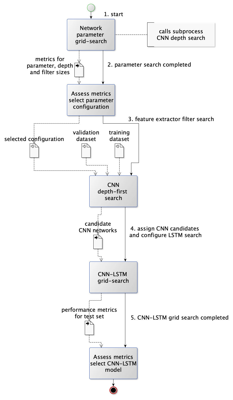
Figure 19 Schematic overview of the development process for the CNN-LSTM model.
Comparative Baseline Models
The CNN-LSTM is compared against three baseline models, the generalised linear model (GLM), random forest (RF) and elastic-net generalised linear model (GLMNET).
The GLM in this study uses the identity link function where \(E\left\lbrack Y \right\rbrack = \eta = X^{T}\beta\), the predictand is assumed to follow the normal distribution, hence is equivalent to the simple linear regression model \(Y = X^{T}\beta\ + \ e\). A full description of the generalised linear model is given in Dobson, 2002 [1]. The GLM model is constructed within the statistical programming environment R (version 4.0.2) [2].
The random forest model constructs an ensemble of multiple trees each grown on a subset of the training data selected at random, resulting estimates are produced by averaging the predictions of all trees. The process of defining a model on the selected subset and averaging the resulting ensemble prediction (termed “bagging”) has the effect of reducing the overall variance of the model estimate given the training data [3]. Trees are grown by considering a set of candidate predictors \(m\) less than the total number of predictors \(p\) at each split and evaluating a splitting criterion function (such as the Gini index) on the “out of bag” sample (a proportion of data not included in the current random subset), as these are selected at random, the combination of all trees are likely to have selected the best choice of predictors [3]. The tuning parameters that influence the performance of the random forest include the number of predictors to consider for each split, the total number of trees to grow, and the maximum number of terminal nodes in each tree. The R package “randomForest” is used in constructing the RF model for this study [4].
The elastic-net GLM applies a penalty term to the coefficient of each of the predictors, in a manner similar to ridge and lasso regression [3]. The estimates for \(\widehat{\beta}\) in each regression method are given as \({\widehat{\beta}}^{\text{ridge}} = \, argmin_{\beta}\left\{ \,\sum_{i = 1}^{N}{\left( y_{i}\, - \,\beta_{0}\, - \,\sum_{j = 1}^{p}{x_{\text{ij}}\beta_{j}}\, \right)^{2}\,} + \,\lambda\sum_{j = 1}^{p}\beta_{j}\, \right\}\,\) and \({\widehat{\beta}}^{\text{lasso}} = \, argmin_{\beta}\left\{ \,\sum_{i = 1}^{N}{\left( y_{i}\, - \,\beta_{0}\, - \,\sum_{j = 1}^{p}{x_{\text{ij}}\beta_{j}}\, \right)^{2}\,} + \,\lambda\sum_{j = 1}^{p}{{|\beta}_{j}|}\, \right\}\) respectively where the \(\lambda\) parameter controls the penalty applied to each coefficient [3]. The elastic-net estimation for \(\widehat{\beta}\) mixes both the ridge and lasso penalties through a parameter \(\alpha\) where the penalty term is defined as \(\lambda\sum_{j = 1}^{p}\left( \alpha\beta_{j}^{2} + \left( 1 - \alpha \right)\left| \beta_{j} \right| \right)\) [3]. With \(\alpha\) closer to \(1\) the penalty acts more like ridge regression whereas with \(\alpha\) closer to \(0\) the penalty acts more like lasso regression. In this study the parameter \(\lambda\) is tuned through k-fold cross validation, with \(\alpha\) been chosen through grid search. The R package “glmnet” provides the procedures for the modelling used in this study [5].
Baseline Model Development
The baseline models were constructed using the following procedure.
A correlation matrix between predictors and predictand was constructed with the training data.
Predictors arranged by strength of correlation.
Each predictor was added to the model one step at a time and metrics were calculated on the validation data set.
Those predictors which increased the \(R^{2}\) metric were retained in the model.
For the random forest, before being able to perform the main correlation search routine, a grid search was performed in order to select the best performing configuration for the number of trees (num_trees), number of terminal nodes (num_nodes) and number of variables to try at each split in the tree for changes in out of bag score (m_try). These were selected using 10-fold cross validation.
A separate GLMNET was trained using 10-fold cross validation for comparison against the GLMNET selected by performing correlation search above. After the search was performed, the GLMNET parameter alpha which is the ratio between the L1 and L2 loss used during parameter smoothing was tuned with a search for the best performing values between 0.1 and 0.9 using 10-fold cross validation (the resulting model is identified as GLMNET ALPHA).
The best performing models for each of the baseline processes are then selected after the search and evaluated against the test set for all sites. Once the best baseline model is determined in the downscaling of a single grid point for each site, the approach is applied in the downscaling of 2-dimensional grid point data, where a single baseline model is constructed for each target radiation output in the 2-dimensional grid. In this case, 81 GLM models are constructed in the 2-dimensional downscaling task (forming a 9x9 set of grid points).
Data formatting for the baseline models requires flattening all features into a single vector, this includes the lagged data points. An additional 11 dummy variables for the month of the year are included in the data frame. Given 71 variables, with an additional 12 lags (852 lagged variables) the number of GCM outputs per record are 923, with the addition of 11 dummy variables for the month encoding there are 934 features per record. In the case of the 2-dimensional downscaling task, there are 9 grid points which are flattened into a single vector, this results in 7739 features per record (9x852+71), with the addition of 11 dummy variables resulting in 7750 feature variables. Table 6 provides the dimensions per record used in developing the baseline models.
| Task | Source Grid Points | GCM variables | Number of Lagged variables | Time variables | Feature Search Space | Target Grid Points | Target Variable | Records \(\mathbf{\times}\) Predictor \(\mathbf{\times}\) Predictand |
|---|---|---|---|---|---|---|---|---|
| 1-d downscaling | \[1 \times 1\] | 71 | \[71\ \times 12\] | 11 | 934 | \[1 \times 1\] | 1 | \[N\ \times 934\ \times 1\] |
| 2-d downscaling | \[3 \times 3\] | 71 | \[71\ \times 12\] | 11 | 7750 | \[9 \times 9\] | 81 | \[N\ \times 7750\ \times 81\] |
Table 6 Dimensions of features and predictands per data set in preparation of baseline modelling.
Deep Learning Modules
Deep learning architectures result from the composition of different modules which are able to learn non-linearities from input data [6]. This study leverages a number of modules, specifically Dense units, the Convolutional module (CNN), the Long Short-Term Memory module (LSTM).
Dense Module
A dense module is simply a layer of the network which contains a number of hidden units each applying a piecewise differentiable activation function \(g\) to the linear combination of input \(I\) with a weight \(W\) and the addition of a bias \(B\). The initial linear combination can be expressed in terms of a matrix multiplication that is then passed as a parameter to the activation function, \(h = g\left( W^{'}I + B \right)\). This is equivalent to the hidden unit of an artificial neural network (deep learning is another name for very large artificial neural networks containing many layers). A differentiable activation function is required for the purposes of back propagation of the error gradient during the optimisation process that is used to train the network. Those functions that are not continuously differentiable (often the family of rectified linear units) are acceptable since the network will not necessarily learn a global minimum of the error gradient, but does reduce the error gradient significantly hence approximates an optimal solution [7]. The activation function allows the network to learn the non-linearities within the data, however dense units are not sparse, since all inputs to a dense layer are connected to every hidden unit by means of a weight. Such a high number of connections means that the dense module has a high number of parameters.
Convolutional Module
In deep learning, the Convolutional module performs many operations in parallel via its application of one or more kernels to different input channels [7]. The kernel is applied such that the same parameters are multiplied with all of the input range, the result is that the learned weights of the kernel are invariant to small local transformations in the input space [7]. Spatial mappings may be captured either globally with respect to the input space or locally, such as in the case where certain features are expected to be limited to specific areas of the input space, the latter is a different form of the convolution operation called "local" or unshared convolution [7]. A compromise between local and global weight sharing is also possible known as tiled convolution, where a set of kernels are learnt for each location in the input, this method allows capturing a small region of local features at each position of the kernel [7]. The direct output of the convolution operation is known as a feature map which is fed into an activation function (known as a detector stage). The activation function in the detector stage may be any of the standard activation functions, however the rectified linear unit (ReLU) is most common. The output of the non-linear activation is then reduced by a pooling operation such as max or average pooling, in order to reduce the sensitivity of the output to shifts and distortions in the input [7]. The convolution operation will result in a reduction of input size after the first convolution, if stride parameters are applied this will reduce the scale of the convolution even further, hence a padding parameter may be applied in order to preserve dimensions. Pooling aggregates the output produced by the convolution and allows the result to remain approximately invariant to small translations in the input [6]. The pooling operation slides over a window of the feature map produced by the output of the non-linear activation. The overall structure of the Convolutional module is illustrated in Figure 20.
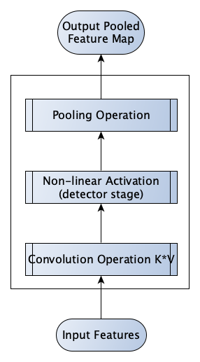
Figure 20 Structure of the Convolutional module, example derived from 47
Long Short-Term Memory Module
A Recurrent Neural Network is a kind of network that can learn the dynamic time dependent relationships within a system by feeding the previous outputs of the network as inputs in subsequent iterations during the training process. However, training such networks proved to be difficult. Recurrent Neural Networks suffered from an issue where the weight gradients of the network units, became very large or extremely small, since the same value was repetitively multiplied with itself over the back-propagation process due to the recurrent structure of the network [7]. The Long Short-Term Memory (LSTM) module introduced self-loops for the output state so as to allow the training process to occur for long durations without reaching extremely high or low values of the weight gradient, in addition, the weight of the loop allows the state (or memory of the unit) to be gated by a forget gate, where a separate hidden unit controls whether a new state is updated or not, and is conditioned as part of the training process [7]. Additional gates are also learnt dynamically, these consist of an input gate, which controls whether to accept input and an output gate which allows the module to learn whether or not to emit output [7]. Each of the gates make use of the sigmoid non-linear activation in order to define an on-off signal, and the input activation can make use of any of the activation functions [7]. The combination of the self-loop and the gate functions allow the LSTM to learn very long term dependencies between inputs, however the state is limited to a single cell [7]. The structure of the LSTM module is illustrated in Figure 21.
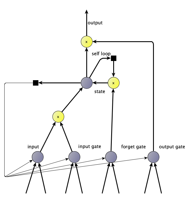
Figure 21 Structure of the LSTM module, example derived from 47.
Learning in Deep Networks
The most common learning procedure, gradient descent, involves an optimisation of weights at each module in response to the propagation of an error gradient, given a loss function. The network is effectively a series of composed functions, and as such, the error gradient results from the application of the chain rule which is progressively nested at each layer in the network. In the simplest case the process can be presented in two parts, a forward pass where activations are computed, and a backward pass where gradients are computed and weights are updated by a small amount in the direction which reduces the error signal. An example of this case is the dense network where each network unit \(j\) at layer \(l\) applies an activation function \(y_{j}^{\left( l \right)} = \phi_{j}\left( v_{j}^{\left( l \right)} \right)\) applied to a linear combination of weights, \(v_{j}^{\left( l \right)} = W_{j}^{\left( l \right)^{T}}Y^{\left( l - 1 \right)}\) [8]. Hence,

At the outer layer, the error, \(e_{j}\), is calculated as the difference between the network estimate \(o_{j}\) and the target variables \(d_{j}\) such that \(e_{j} = d_{j} - o_{j}\). In order to calculate the gradient at a given layer, the product between the error signal of the layer above (or error at the output layer) and the derivative of the activation function with respect to its inputs is used [8].

Weights at each layer are then updated in the direction of the gradient scaled by the learning rate \(\eta\) [8].
\[w_{\text{ji}}^{l} = w_{\text{ji}}^{l} + \eta\delta_{j}^{\left( l \right)}y_{i}^{\left( l - 1 \right)}\]
Variations include modification of the learning rate during the learning iterations \(n\) and the addition of parameters for momentum \(\alpha \in \left\lbrack 0,1 \right\rbrack\), which encourages the weights to move in the direction of previous updates [8].
\[w_{\text{ji}}^{l}\left( n \right) = w_{\text{ji}}^{l}\left( n \right) + \alpha\left\lbrack w_{\text{ji}}^{l}\left( n - 1 \right) \right\rbrack + \eta\delta_{j}^{\left( l \right)}y_{i}^{\left( l - 1 \right)}\left( n \right)\]
The procedure of gradient descent is detailed extensively in sources such as Haykin [8], Goodfellow, et al. [7] and Strang [9].
Choice of Architecture
This study initially investigated the use of several architectures discussed in the literature review, of particular interest were the SRCNN super resolution network as described in Caballero, et, al. [10] the Conv-LSTM network as described by Shi, et al. [11] and the CNN-LSTM hybrid network as described by Ghimire et, al. [12].
After an initial experimentation process the 2-dimensional Convolutional models, such as the SRCNN, and the Conv-LSTM architectures, did not produce metrics that indicated suitable mapping between outputs and downscaled observations and exhibited low \(R^{2}\) and negative efficiency scores. After these initial experiments it was decided that the thesis will focus on the use of the CNN-LSTM architecture in the task of local and universal downscaling, which leverages a 1-dimensional convolution rather than 2-dimensional.
The Python programming language (version 3.8.2) [13] and the Tensorflow library (version 2.3.0) [14] are utilised by this thesis in the implementation of the deep network architectures.
Proposed Model Development
The proposed model is a variant of the CNN-LSTM architecture and is trained on the lagged month averaged data, consisting of a lag for 12 months of GCM predictors in both the 1-dimensional and 2-dimensional downscaling tasks. Aside from the dummy encoded month data, two additional features were added for cosine and sine encoded representation for the day of year (13 time variables). In the case of 1-dimensional convolution, data is formatted with 2-dimensions being the number of time steps (depth-wise) and the number of predictors (column wise). During training a third dimension is added representing the number of examples that are presented to the network as a batch of data (the batch size). The dimension of the input is (batch size \(\times\) time steps \(\times\) predictors).
The resulting dimensions are:
- (batch size = 128, time steps = 12, predictors = 84)
In the case of the 2-dimensional downscaling task, a 1-dimensional convolution is applied where all grid points are flattened into 9 grid points \(\times \ (71\ + \ 13)\) feature vector, with 12 lagged months (time steps) per frame with the batch size of 64.
The resulting dimensions are:
- (batch size = 64, time steps = 12, predictors = 652)
| Task | Source Grid Points | GCM Variables | Lagged Variables | Time Variables | Feature Search Space | Target Grid Points | Target Variable |
Records \(\mathbf{\times}\) Batch \(\mathbf{\times}\) Predictors \(\mathbf{\times}\)Timesteps \(\mathbf{\times}\) Predictand |
|---|---|---|---|---|---|---|---|---|
| 1-d downscaling | \[1 \times 1\] | \[71\] | \[71 \times 12\] | \[13\] | \[84 \times 12\] | \[1 \times 1\] | \[1\] | \[N \times 128 \times 84 \times 12 \times 1\] |
| 2-d downscaling | \[3 \times 3\] | \[71\] | \[71 \times 12\] | \[13\] | \[652 \times 12\] | \[9 \times 9\] | \[81\] | \[N \times 64 \times 652\ \times 12\ \times 81\] |
Table 7 Dimensions of data required for CNN-LSTM model development.
Given the large feature space, regularisation is applied at each layer in order to encourage a reduction in the weights associated with features that do not contribute to the overall accuracy of the model.
The diagram in Figure 22, illustrates the architecture of the CNN-LSTML network demonstrating the general structure of each module. Note that the structure of the below network shows four convolution modules, whereas the number of intermediate convolution modules in the final network was selected via grid search performed prior to end to end training. Batch normalisation and max-pooling were determined to be effective for the CNN modules as a result of the grid search, however batch normalisation was not enabled on the output layer.
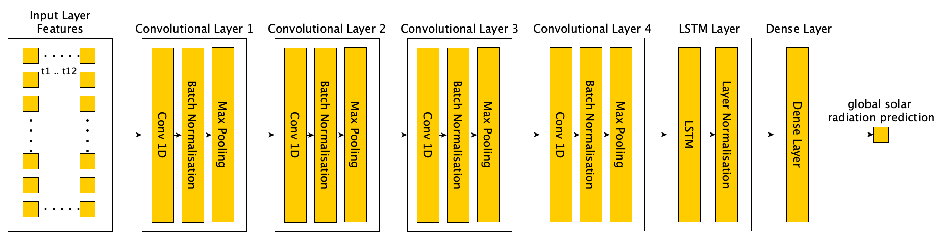
Figure 22 Conceptual overview of the CNN-LSTML architecture.
A second network was constructed (CNN-LSTML DENSE) to extend upon the above architecture, in this architecture the output layer consisted of a copy of the input layer as well as the additional radiation target variable. The network was trained to replicate the input values, as well as to predict the radiation variable. This architecture was designed so as to test whether replicating the input enabled the network to learn an additional mapping to the target radiation. The architecture is shown in Figure 23.
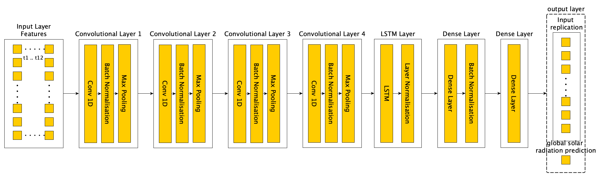
Figure 23 Conceptual architecture of CNN-LSTML DENSE network.
The same architecture is applied in the 2-dimensional downscaling, with the exception that the number of input features are increased to accommodate the 9 individual grid points for the GCM output variables, and the output layer provides a prediction for each of the 81 radiation grid points instead of a single radiation grid point. Figure 24 illustrates the architecture for the CNN-LSTMU model developed in the 2-dimensional downscaling task.
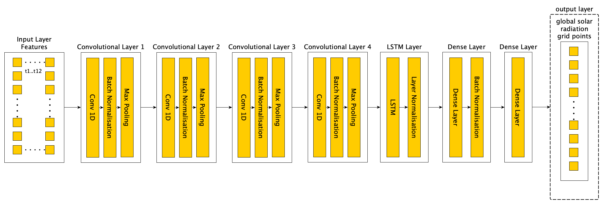
Figure 24 Conceptual CNN-LSTMU architecture as applied to the 2-dimensional grid downscaling task.
CNN Network Search Procedure
The optimal network architecture is not known before training, similarly there are a number of hyper-parameters whose optimal values are not known prior to training. A search procedure is required in order to identify the best range of configurations to use when developing the network architecture against the selected data set. The search procedure involved a grid search for the optimal configuration of 1-dimensional CNN filters prior to the final grid search within the LSTM architecture. This was a depth first greedy search between 1 and 10 modules (computational memory and resources permitting) over a short run of 1000 epochs for a single site. The number of filters at each layer ranged between 50 to 1000 filters, with a kernel size held at 3 and a stride parameter held at 1 (following the design intuition outlined in Hasanpour, et al. [15].
The search procedure is summarised as follows.
Set the filter sizes collection to empty.

For i in 1 to max_depth
 Set the current layer to i.
 Set the current depth score to 0
 Set the best filter at depth i to 0
 For j in 50 to 1000 filters step by 50
  Build network with depth i using the filter sizes collection.
  Add CNN module with j filters to network.
  Train network and evaluate on validation data set.
  If R^2 is greater than current depth score then
   Set best filter at depth i to j
   Set current depth score to R^2
  End
 End
 Append best filter at depth i to previous filters collection
End
Table 8 Summary of CNN filter size search procedure.
The above process constructs multiple CNN layers and progressively selects the best filter size at each layer based on the \(R^{2}\) metric. The procedure is invoked as a subprocess during the grid search for parameters and during the second stage search when searching for the depth and filter configuration of the CNN modules within the architecture. The resulting sequence of filter sizes are then evaluated and added to a candidate set of CNN configurations for use in the LSTM grid search. The grid search is performed multiple times against a single site in order to determine the best configuration. A subsequent grid search is performed in order to evaluate parameterisations of further network configurations shown in Table 9.
| Network Feature | Configuration | Description |
|---|---|---|
| Max Pooling | On or Off | Determine the performance of max-pooling after each CNN module. |
| Max pooling followed by Dropout | On or Off | Determine the performance of max-pooling followed by dropout after each CNN module. |
| 1 Time step versus 12 timesteps | Timesteps = [1, 12] | Determine the performance of the CNN when evaluated against 1 timestep containing lagged variables versus 12 timesteps with no lagged variables in each row. |
| Batch normalization after output. | On or Off | Determine the effect of batch normalisation after output module. |
| L2 vs L1 regularization | L1 or L2 | Determine the effect of using L2 versus L1 regularization in the network architecture. |
| Batch Size 32 vs 128 | Batch Size = [32, 128] | Determine the effect in batch size on training. |
| Narrow feature maps versus wide feature maps. |
For narrow feature maps filters were constrained between 10 and 100. For wide feature maps filters were constrained to allow 20 units and the range 50 to 1000 with steps of 50 units. |
Determine whether a deeper network with smaller filters would be more effective than a shallower network with wider filters. |
| Include predictors based on best predictors selected from GLM training. | Predictors derived from best GLM model. |
Determine whether pre-selection of predictors based on the performance of a simpler model is effective in improving performance of the CNN. Note the L1, L2 regularization determines which predictors are influential within the CNN pipeline. |
Table 9 Table of network configuration parameters evaluated during search procedure.
A number of candidate architectures were selected as a result of the grid search on the CNN and were then selected as candidates for the CNN-LSTM architecture. The \(R^{2}\) metric was used as an indicator of whether the configuration improved the performance of the network at the associated depth. Each of the configurations defaulted to batch normalisation and L1 regularization unless indicated. The box plot in Figure 25 shows the range of the metric for each configuration at the corresponding depth, the \(R^{2}\) metric is shown in Table 10 up to depth 4.
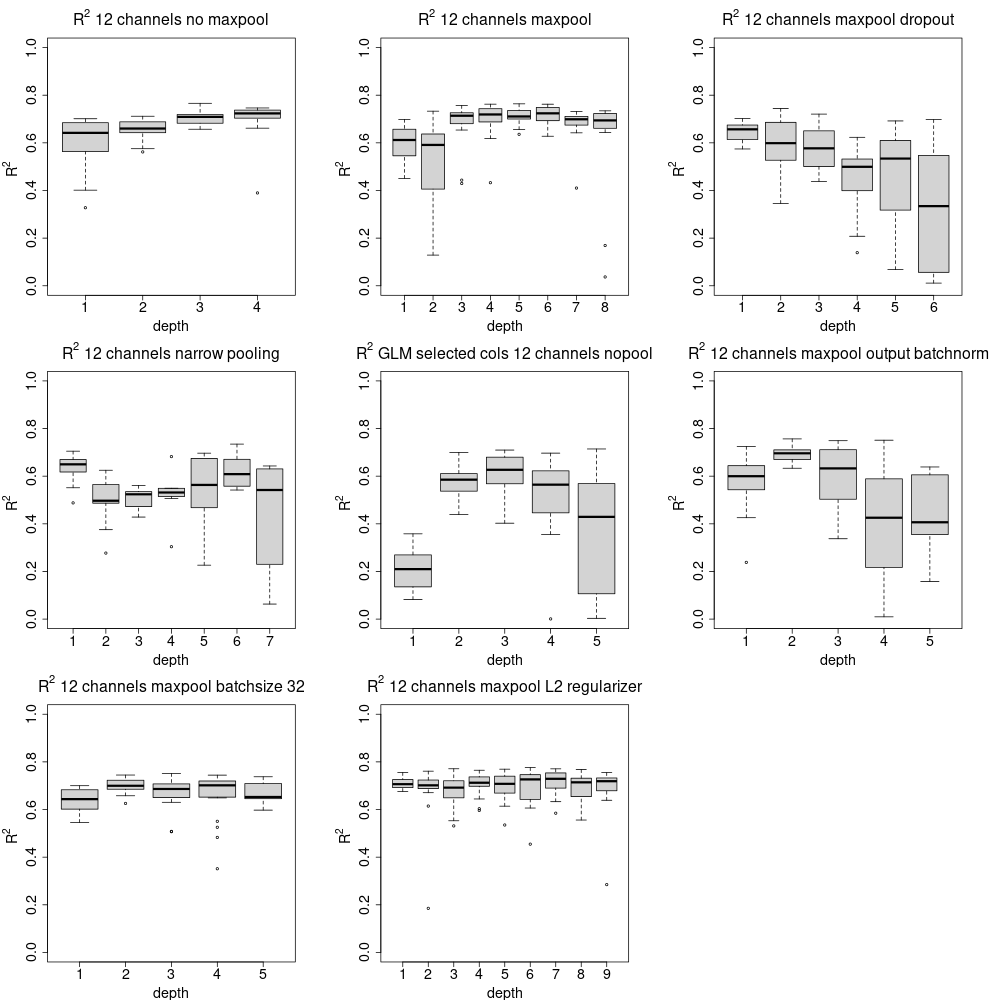
Figure 25 Boxplot of \(R^{2}\) resulting from comparison of different parameter combinations during the CNN search process. Comparisons determined that a 12 timestep CNN with max pooling and L2 regularization was the preferred configuration for the CNN architecture. Performance remained relatively constant and became more variable as the depth of the CNN increased.
| Configuration | \(\mathbf{R}^{\mathbf{2}}\) Depth 1 | \(\mathbf{R}^{\mathbf{2}}\) Depth 2 | \(\mathbf{R}^{\mathbf{2}}\) Depth 3 | \(\mathbf{R}^{\mathbf{2}}\) Depth 4 |
|---|---|---|---|---|
| Max Pool | 0.70 | 0.73 | 0.76 | 0.76 |
| Max Pool Batch Size 32 | 0.70 | 0.74 | 0.75 | 0.74 |
| Max Pool Dropout | 0.70 | 0.74 | 0.72 | 0.62 |
| Max Pool L2 regularisation | 0.76 | 0.76 | 0.77 | 0.76 |
| Max Pool Output Layer Batch Normalisation | 0.72 | 0.76 | 0.75 | 0.75 |
| Narrow Filters with Pooling | 0.70 | 0.62 | 0.56 | 0.68 |
| No Max Pooling | 0.70 | 0.71 | 0.77 | 0.75 |
| GLM Selected Columns No Pooling | 0.36 | 0.70 | 0.71 | 0.70 |
Table 10 Average \(R^{2}\) and Depth for each Network Configuration. Bolded values indicate better scores.
As a result of the parameter search, it was determined that L2 regularisation was more effective than L1 regularisation in this setting, and that the use of drop-out resulted in higher variance in the \(R^{2}\) metric. max-pooling on Convolutional layers resulted in a better \(R^{2}\) metric, and that constraining the number of filters (between 10 and 100) during the search did not result in as high \(R^{2}\) on average as opposed to permitting a larger number of filters (between 20 and 1000). Disabling batch normalisation on the output layer produced \(R^{2}\) that was less variable than otherwise enabling it. However, batch normalisation was enabled on intermediate layers.
Combined CNN-LSTM Grid Search Procedure
The selected CNN-LSTM architecture was then determined through iteratively training the resulting CNN modules selected from the best performing configurations of the previous search. The CNN-LSTM search iterates over the parameters listed in Table 11.
| Parameter | Description | Parameterisation |
|---|---|---|
| Filter size of Convolutional Layers | The set of filter sizes to evaluate during end to end CNN-LSTM training. | Determined by CNN module grid search. |
| Kernel Size of Convolutional Layers | The width of the convolution kernel. | 3, 5, 7 |
| Convolution Stride | The search was performed with a fixed stride parameter. | 1 |
| LSTM Internal Units | The number of units within the recurrent module. | 12, 32, 64, 128 |
| Learning Rate and Epochs | Alter the learning rate and number of epochs to determine influence on performance. | 0.01 to 10^-5 |
| Momentum | Alter the momentum for the RMSprop optimization procedure to determine influence on performance. | 0.01 to 10^-5 |
| Loss Function | Evaluate the use of Mean Squared Error Loss or Mean Absolute Error Loss | MAE or MSE |
Table 11 Parameters for end to end training of CNN-LSTM module.
Selected Models for Downscaling Average Monthly Radiation
After training the candidate models, an assessment based on the evaluation metrics is carried out in order to compare baseline models to the proposed models. Table 12 lists the final configuration for each of the selected models resulting from each respective search procedure.
| Model Name | Parameterisation | ||||||||||||||||||||||||||||||||||||
|---|---|---|---|---|---|---|---|---|---|---|---|---|---|---|---|---|---|---|---|---|---|---|---|---|---|---|---|---|---|---|---|---|---|---|---|---|---|
| GLM - General Linear Model with Gaussian link function. |
|
||||||||||||||||||||||||||||||||||||
| GLMNET - Elastic Net with Gaussian Link Function |
|
||||||||||||||||||||||||||||||||||||
| GLMNET_ALPHA – Elastic Net with Gaussian Link Function and tuned Alpha parameter. |
|
||||||||||||||||||||||||||||||||||||
| RF – Random Forest |
|
||||||||||||||||||||||||||||||||||||
| CNN-LSTML – 1-d Convolutional LSTM model. |
|
||||||||||||||||||||||||||||||||||||
|
CNN-LSTML DENSE 1-d Convolutional LSTM model with dense layer for multiple variables. |
|
||||||||||||||||||||||||||||||||||||
| GLM Universal Model |
|
||||||||||||||||||||||||||||||||||||
|
CNN-LSTMU 2-d Universal Convolutional LSTM model for 2-dimensional downscaling. |
|
Table 12 Parameterisation of Models resulting from search and training procedures.
References

Downscaling Global Climate Models with Convolutional and Long-Short-Term Memory Networks for Solar Energy Applications by C.P. Davey is licensed under a Creative Commons Attribution-NonCommercial-ShareAlike 4.0 International License.